Beyond-GCR access

Beyond-GCR access#

Owners: PatriciaLarsen @plarsen
Last Verifed to Run: 2024-06-04 (by @plarsen)

This notebook will show you how to access the DP0.2 object catalog directly through the parquet files at nersc, using the Generic Catalog Reader (GCR, yymao/generic-catalog-reader) to access the file locations and metadata. We will discuss why you may want to do this, and how to do some basic tasks efficiently.

Learning objectives:

After going through this notebook, you should be able to:

Access the DP0.2 object catalog directly using parquet functions for more advanced read-in options

Future additions:

Get the SRV filters
Add join with truth tables here and some more examples of advanced use cases

Logistics: This notebook is intended to be run through the JupyterHub NERSC interface available here: https://jupyter.nersc.gov. To setup your NERSC environment, please follow the instructions available here: https://confluence.slac.stanford.edu/display/LSSTDESC/Using+Jupyter+at+NERSC

Why do this?#

There are two main reasons we’re providing this information.

Firstly while we can provide a straightforward read method using the GCR, this has been developed with the intention of being agnostic to data format. However for the object catalogs we can expect these will stay in parquet format, and we find that some DESC members want access to methods which they can access through the parquet file paths or handles, which are not easily translated to other data formats.
Secondly there’s a question of choice and ease. Some codes may work with direct parquet reads and rewriting them to use the GCR may not be time-effective, and people who are comfortable using parquet files may prefer direct access to better optimize and understand what they’re doing.

%matplotlib inline
import numpy as np
import matplotlib.pyplot as plt
import sys
import pyarrow.compute as pc
import pyarrow.dataset as ds
from GCR.utils import concatenate_1d

import time

Accessing the object catalog metadata with the GCR#

The GCRCatalogs package is a DESC project which aims at gathering in one convenient location various simulation/data catalogs made available to the collaboration.

Here we will show you how to access the information on the direct parquet handles and file locations available through the GCR, for the object catalogs from DC2 Run2.2i that the Rubin project ran using the DMStack, DP0.2 (data preview 0.2).

sys.path.insert(0,'/global/cfs/projectdirs/lsst/groups/SRV/gcr-catalogs-test')
import GCRCatalogs

# Load the object catalog
catalog = GCRCatalogs.load_catalog('lsst_object_full')

A significant numbers of cosmology catalogs besides the DP0.2 object catalogs are also available through the GCR, use sorted(GCRCatalogs.get_available_catalogs(False)) to see a full list and visit the DC2 Data Product page to see all the DC2-related catalogs.

DP0.2 object catalog Schema#

The quantities available in the catalog can be found on the project website here: https://dm.lsst.org/sdm_schemas/browser/dp02.html, but we can also access these from the GCR in the following way. Note that these methods are equivalent, for this specific catalog named lsst_object we have done no quantity translation and so it’s safe to assume that these follow the lsst conventions exactly.

Note that for comparisons between the DP0.2 and DC2 object catalogs you may prefer to use a translation layer to convert the DP0.2 catalog into DC2 conventions before read-in, this is available by using dp02_object rather than lsst_object. We will cover the use of the translated catalog in a different tutorial.

quantity_list = sorted(catalog.list_all_native_quantities())
for i in range(4):
    q = quantity_list[i]
    info = catalog.get_quantity_info(q)
    print(q)
    print('------------------')
    print(info['description'])
    print('Type: ' + info['type'] + ',', 'Units: ' + info['unit'])
    print(' ')

coord_dec
------------------
Fiducial ICRS Declination of centroid used for database indexing
Type: double, Units: deg
 
coord_ra
------------------
Fiducial ICRS Right Ascension of centroid used for database indexing
Type: double, Units: deg
 
deblend_nChild
------------------
Number of children this object has (defaults to 0)
Type: int32, Units: none
 
deblend_skipped
------------------
Deblender skipped this source
Type: boolean, Units: none
 

Methods to access this dataset#

First let’s show you how to use GCR to directly access the Parquet file handle. This handle is simply opening the Parquet file as in the code snippet that follows. If there is a use-case in which you need a different access method the file path is also available

import pyarrow.parquet as pq

handle = pq.ParquetFile(self.path)

for parquet_data in catalog._datasets[:2]:
    print('Dataset info: ', parquet_data.info)
    print('Dataset handle: ', parquet_data.handle)
    print('Dataset path: ', parquet_data.path)
    print(' ')

Dataset info:  {'tract': 2897}
Dataset handle:  <pyarrow.parquet.core.ParquetFile object at 0x7fb28af00d00>
Dataset path:  /global/cfs/cdirs/lsst/shared/rubin/DP0.2/objectTable/objectTable_tract_2897_DC2_2_2i_runs_DP0_2_v23_0_1_PREOPS-905_step3_1_20220317T233937Z.parq
 
Dataset info:  {'tract': 2898}
Dataset handle:  <pyarrow.parquet.core.ParquetFile object at 0x7fb28aa503d0>
Dataset path:  /global/cfs/cdirs/lsst/shared/rubin/DP0.2/objectTable/objectTable_tract_2898_DC2_2_2i_runs_DP0_2_v23_0_1_PREOPS-905_step3_1_20220308T153907Z.parq
 

Format notes#

you need to know which filter notation you need, in this case we use pyarrow.compute filters. There’s a conversion script between string filters and pyarrow.compute filters below for convenience

Let’s first try an iterative read (reducing memory requirements) and concatenate the results

time_start = time.time()

# take the file handles and combine them into a dataset
sources = [parquet_data.path for parquet_data in catalog._datasets]
dataset = ds.dataset(sources)

filter = pc.field('detect_isPrimary')&(pc.field("r_ra") > 0) & (pc.field("r_decl") < -40)

ra_full = []
dec_full = []
for batch in dataset.to_batches(columns=["r_ra","r_decl"], filter=filter,):
    ra_full.append(batch["r_ra"])
    dec_full.append(batch["r_decl"])
time_end = time.time()
ra_full = concatenate_1d(ra_full)
dec_full = concatenate_1d(dec_full)

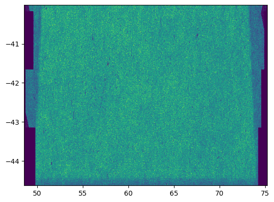
plt.hist2d(ra_full,dec_full,bins=1000)
plt.show()
print(round(time_end-time_start), 'seconds to read data')

../../_images/d9a2de576ea1a7a6e16b3fe83e8e4629829d80f84d82f5d55270724f364433ed.png

13 seconds to read data

and then a full read into a pyarrow table format (you can just use a .to_pandas() to convert it to a pandas table if you prefer those)

time_start = time.time()

# take the file handles and combine them into a dataset
sources = [parquet_data.path for parquet_data in catalog._datasets]
dataset = ds.dataset(sources)

filter = pc.field('detect_isPrimary')&(pc.field("r_ra") > 0) & (pc.field("r_decl") < -40)
data = dataset.to_table(columns=["r_ra","r_decl"], filter=filter,)

time_end = time.time()

plt.hist2d(data['r_ra'],data['r_decl'],bins=1000)
plt.show()
print(round(time_end-time_start), 'seconds to read data')

pandas_data = data.to_pandas()

7 seconds to read data

Creating filters#

If you’re not familiar with pyarrow filters or have a big string of GCR filters and want a conversion script the below should work

import re
import numexpr as ne

def convert_to_pyarrow_filter(filter_list):
    for i in range(len(filter_list)):
        for n in set(ne.necompiler.precompile(filter_list[i])[-1]):
            filter_list[i] = re.sub(rf"\b({n})\b", "pc.field(\"\\1\")", filter_list[i])
    total_query = eval(filter_list[0])
    
    if len(filter_list)>1:
        for i in range(1,len(filter_list)):
            total_query = total_query&eval(filter_list[i])
    return total_query
    
convert_to_pyarrow_filter(['detect_isPrimary', "r_ra > 0", "r_decl < -40"])

<pyarrow.compute.Expression ((detect_isPrimary and (r_ra > 0)) and (r_decl < -40))>

time_start = time.time()

# take the file handles and combine them into a dataset
sources = [parquet_data.path for parquet_data in catalog._datasets]
dataset = ds.dataset(sources)

filter = convert_to_pyarrow_filter(['detect_isPrimary', "r_ra > 0", "r_decl < -40"])
data = dataset.to_table(columns=["r_ra","r_decl"], filter=filter,)

time_end = time.time()

plt.hist2d(data['r_ra'],data['r_decl'],bins=1000)
plt.show()
print(round(time_end-time_start), 'seconds to read data')

2 seconds to read data

Advanced tools#

With parquet datasets you can use some more advanced tooling through the compute tool. Let’s say you want to combine two datasets, like the object catalog and the truth match catalog. You can do that through the join function.

import pyarrow.dataset as ds

ds1 = ds.dataset(table1) ds2 = ds.dataset(table2)

joined_ds = ds1.join(ds2, key=”id”)

You can create a scanner over the data, where the scanner doesn’t run immediately but exposes the ability to run and then apply other methods. This can be especially useful for applying extra filters.

dataset.scanner(filter=ds.field(“year”) > 2020).to_table()

You can acess the acero framework to do operations over batched data in an efficient way (which underlies the dataset methods). But if you do so you should note that:

“Acero is not intended to be used directly by data scientists. It is expected that end users will typically be using some kind of frontend. For example, Pandas, Ibis, or SQL. The API for Acero is focused around capabilities and available algorithms. However, such users may be interested in knowing more about how Acero works so that they can better understand how the backend processing for their libraries operates.”