Effect: Tree rings

During the growing of silicon boules the doping percentage can vary over time building “tree-ring” like structure in doping concentration. Much like a n-p junction, the gradient in doping establishes a static lateral electric field causing electrons to drift laterally into adjacent pixels while traveling through the silicon bulk. It leads to position-dependent distortions of the images, as well as to periodic intensity variations in flat fields.

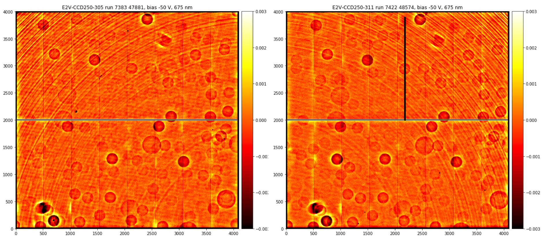
Typical tree rings seen in flatfields

For a more thorough introduction see e.g. Okura et al. (2015).

Contact person(s) if any:

Craig Lage, Mike Jarvis, Andrei Nomerotski/SAWG

Reference Material:

See recent talk by Craig Lage here

Tree rings analysis using BNL data by Sergey Karpov is here

Another review of tree rings in BNL sensors by Hye-Yun Park is here

Data Provenance:

The model is validated using the data acquired at BNL on TS3 (30 ITL, 37 E2V sensors, 106 runs in total) and on TS8 (39 ITL, 72 E2V sensors, 496 runs in total).

All data are available on ASTRO cluster in BNL at: /gpfs01/astro/workarea/ccdtest/prod

The model parameters

Model Details:

The tree rings are typically seen in flat field images where they represent the effective pixel area variation (or the Jacobian of coordinate transformation). On the other hand, for efficient simulation of data the coordinate distortion function is necessary. Therefore, it is decided to build an analytical model for radial coordinate displacement, and then compute pixel area variation from it.

The following model is selected to represent the effect:

\[\delta r = \left( \sum \sin(\omega_i r + \phi_i)/\omega_i - \sum \cos(\omega_i r + \phi_i)/\omega_i\right) \cdot (A+Br^4)\]

Polynomial term describes the increase of tree rings amplitude with moving away from the center. Corresponding area variation is then

\[\delta S = \left( \sum \cos(\omega_i r + \phi_i) + \sum \sin(\omega_i r + \phi_i)\right) \cdot (A+Br^4)\]

The parameters are chosen based on data acquired by Hye-Yun Park on TS3 for 5 ITL and 1 E2V sensors, available here.

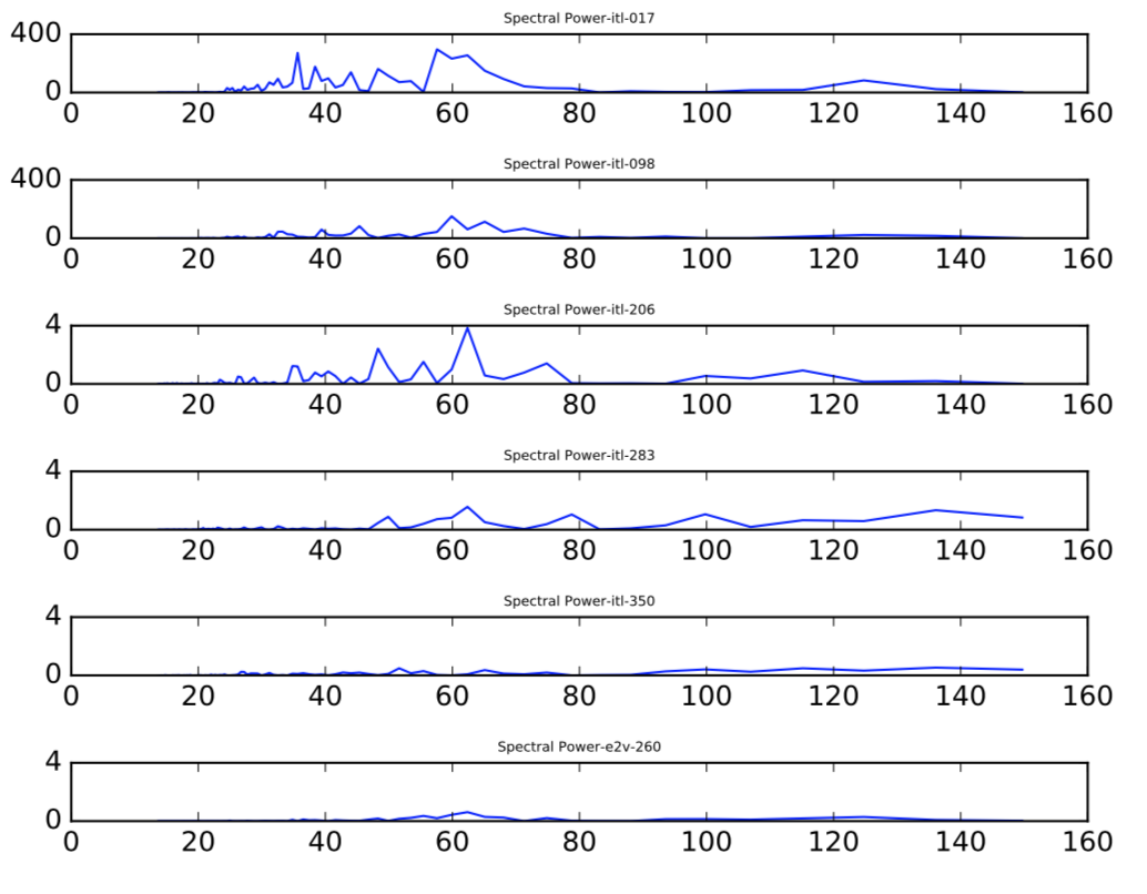
Input data used for selection of tree ring parameters

The parameters are randomly generated for all sensors using build_tree_ring_file.py script according to the following rules:

• 15 sine + 15 cosine frequencies (with random phases) normally distributed with mean 60 pix and sigma 10 pix

• 5 sine + 5 cosine frequencies (with random phases) normally distributed with mean 35 pix and sigma 10 pix

• 60% sensors have small amplitudes, 40% - large (order of magnitude larger) amplitudes, uniformly distributed with ~2 times spread.

Actual parameters pre-generated for all sensors are stored in tree_ring_parameters_2018-04-26.txt. The code in imsim/tree_rings.py reads this file, constructs radial displacement function and passes it to galsim.SiliconSensor constructor in galsim/sensor.py. Then the low-level C++ code in Silicon.cpp uses it for actual displacement of incoming photons, applying also conversion depth correction to it (so the electrons converted deeper have smaller displacement). The latter is handled by Silicon::insidePixel method.

Validation Criteria:

The validation is based on an uniform analysis of flat fields from large set of CCDs studied at BNL on TS3 and TS8. The superflats have been created from all available flat field frames, and then processed using the code published here. Processing consisted of high-pass filtering of superflats, artefact and noise masking, automatic determination of tree rings center, and derivation of an angle-averaged relative intensity variation as a function of radius.

The simulated data have been generated for all 189 different imSim sensor configurations using analytic formulae for pixel area variations shown above.

The following criteria are used for comparison of simulated and experimental data:

• Visual comparison of flat fields

• Average periodograms

• Radius-dependent frequency structure (radius-resolved periodogram)

• Distribution of amplitudes at fixed radius

• Radial dependence of amplitude, estimated through sliding window sample variance corrected to sine wave amplitude using sqrt(2) coefficient.

Validation Results:

Simulated flat fields

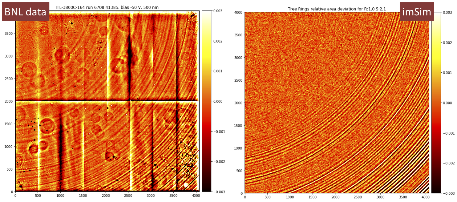
Comparison of simulated flats to actual ITL sensor data

Simulated flat field (right) looks quite similar to the actual one acquired on TS3 at BNL (left). Color-coded are relative intensity variations corresponding to effective pixel area changes due to electron displacement.

Average periodograms

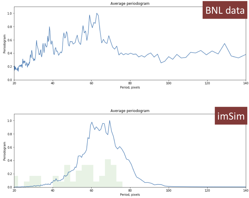
Comparison of periodograms of simulated and actual data

Average periodograms of simulated data (lower) are generally consistent with experimental data (upper panel) except for a slight shift of main peak to longer periods and the absence of lower-period excess seen in actual data. The latter is despite the presence of actual frequencies there in simulation (see overplotted histogram of simulated frequency components in the lower panel).

Radius-resolved periodograms

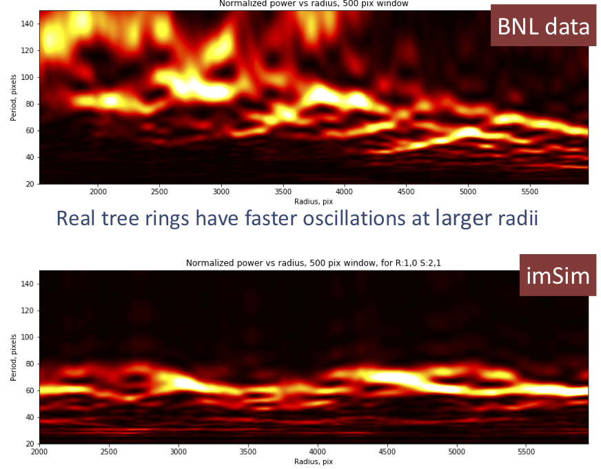
Comparison of radius-resolved periodograms of simulated and actual data

Radius-resolved periodograms of actual data (upper) show signs of an evolution of primary frequencies with radius - on smaller radii periods of oscillations are larger, tree rings appear “smoother” than on larger radii. This may also be seen visually in the flat fields above. Radius-resolved periodograms of simulated data are flat, as expected from the underlying model.

Amplitudes at fixed radius

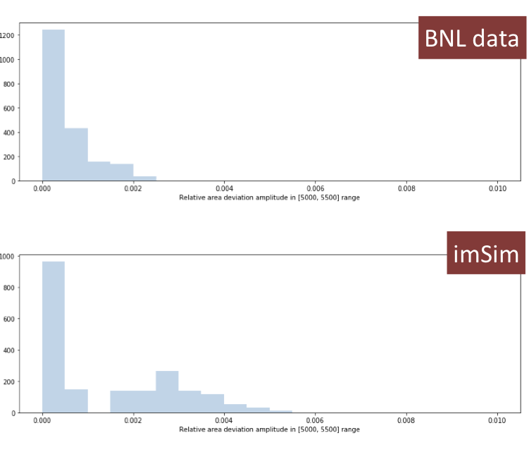
Comparison of amplitudes of simulated and actual data

Amplitudes estimated as a sample variance between 5000 and 5500 pixels radii (multiplied by sqrt(2) to convert to sine wave amplitude) of simulated data (lower panel) show characteristic two-peak structure due to underlying model which includes 60% lower-amplitude sensors and 40% higher amplitude ones. Actual experimental data (upper) show smooth, continuous distribution of amplitudes instead, with smaller amount of higher amplitude sensors than simulated.

Radial dependence of amplitudes

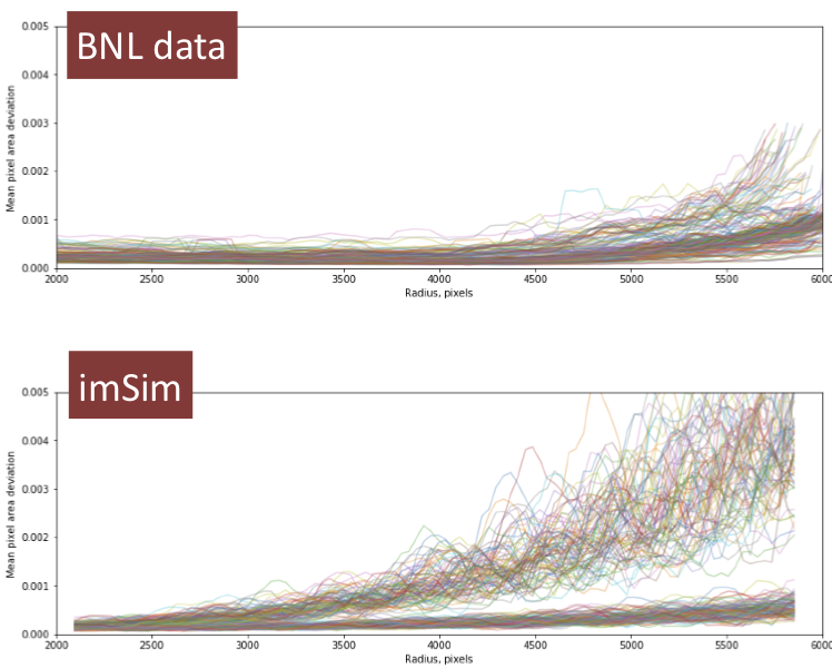
Comparison of radial amplitudes of simulated and actual data

Radial dependence of aplitude, estimated by a sliding window sample variance (multiplied by sqrt(2) to convert to sine wave amplitude) of simulated data (lower) show the same characteristic two sets distribution due to underlying model. It also shows generally smoother growth with radius than experimental data (upper) - experimental data seem to grow faster with radius, probably with polynomial degree larger than 4 used in the model.

Conclusions

Overall properties of simulated tree rings look qualitatively similar to actual ones of sensors measured at BNL, with some minor properties missing (radial dependence of primary frequencies, radual dependence of amplitudes).

Relevant Project Team for input if any:

Camera

Release and approval log:

03/30/18 - Initial Version - CWW

08/11/18 - Updated version with more details on model and validation - Sergey Karpov