Streamobs: generate stream mocks#

Generate stellar stream mock catalogs from configuration files and complete existing tables with missing columns. Streamobs allows sampling of the following quantities:

(phi1, phi2): stellar coordinates in the stream frame
dist: distance modulus of stars
{survey}_{band}: apparent magnitude in a given photometric band of a chosen survey

Future versions may also include sampling of proper motions and velocities.

Streamobs can further convert these intrinsic quantities into observed quantities. For more details, see the notebook tutorial_inject_stream.ipynb.

In this tutorial, you’ll learn to:

Define model components: density, track, distance modulus, isochrone
Build or load a configuration and sample a mock catalog
Complete partial catalogs (e.g., by adding magnitudes)

import sys
import os
import pandas as pd
import yaml
import numpy as np
import matplotlib.pyplot as plt
import scipy

# Import necessary modules form streamobs
%load_ext autoreload
%autoreload 2
from streamobs.utils import parse_config
from streamobs.model import StreamModel

1) Build a stream configuration#

To set up a stream model, we use a configuration file or dictionary that defines all necessary components. It can include:

density – samples phi1 values along the stream
track – gives phi2 as a function of phi1 (center + spread, using a Gaussian or Uniform sampler)
distance_modulus – defines \(DM(phi1)\) for computing apparent magnitudes
isochrone – samples the color–magnitude diagram (required to generate magnitudes)

You can choose how each quantity depends on phi1 (e.g., constant, linear, spline, etc.).

Notes:

To generate magnitudes, you need at least both dist and isochrone.
The velocity model is currently a placeholder (returns NaN).
Samplers and functions are selected using the type keyword (e.g., "Uniform", "CubicSplineInterpolation").

# Build a config dictionary directly

config = {
    # Density model
    "density": {"type": "Uniform", "xmin": -9.0, "xmax": 9.0},
    # Track model
    "track": {
        "center": {
            "type": "Constant",
            "value": 0.0,
        },  # center line of the stream in degrees
        "spread": {"type": "Constant", "value": 0.2},  # spread of the stream in degrees
        "sampler": "Gaussian",
    },  # how to sample across the stream
    # Isochrone model
    "isochrone": {
        "name": "Marigo2017",  # isochrone set name
        "survey": "lsst",  # survey for filter set
        "age": 12.0,  # Age in Gyr of the population
        "z": 0.0006,  # Metallicity of the population
        "band_1": "g",  # first band for color-magnitude
        "band_2": "r",  # second band for color-magnitude
        "band_1_detection": True,
    },
    # Distance modulus model. Here an example of a constant distance modulus
    "distance_modulus": {
        "center": {"type": "Constant", "value": 16.5},
        "spread": {"type": "Constant", "value": 0.0},
    },
}

# or load from a config file
# config_path = os.path.join(base_dir, 'config', 'toy1_config.yaml')
# config = parse_config(config_path)['stream']

print(config)

{'density': {'type': 'Uniform', 'xmin': -9.0, 'xmax': 9.0}, 'track': {'center': {'type': 'Constant', 'value': 0.0}, 'spread': {'type': 'Constant', 'value': 0.2}, 'sampler': 'Gaussian'}, 'isochrone': {'name': 'Marigo2017', 'survey': 'lsst', 'age': 12.0, 'z': 0.0006, 'band_1': 'g', 'band_2': 'r', 'band_1_detection': True}, 'distance_modulus': {'center': {'type': 'Constant', 'value': 16.5}, 'spread': {'type': 'Constant', 'value': 0.0}}}

# Create stream model and generate stars
stream_model = StreamModel(config)
stream_df = stream_model.sample(4500)

# The dataframe contains: phi1, phi2, distance, magnitudes, etc.
print(f"✓ Generated {len(stream_df)} stars")
print("\nFirst 5 stars:")
print(stream_df.head())

✓ Generated 4500 stars

First 5 stars:
       phi1      phi2  dist   mu1   mu2    rv  lsst_g_true  lsst_r_true  \
4.739512  0.015756  16.5  None  None  None    28.982359    27.582928   
-1.499554 -0.343139  16.5  None  None  None    27.581603    26.354772   
8.207016 -0.176948  16.5  None  None  None    26.265005    25.228614   
0.680482 -0.088033  16.5  None  None  None    27.004769    25.868177   
4.064195  0.077374  16.5  None  None  None    27.373922    26.179369   

       mass  
0.158219  
0.246747  
0.387048  
0.299648  
0.265148  

# Quick look: sky track, 1D density, CMD
fig, ax = plt.subplots(1, 3, figsize=(16, 5))

# Stream on the sky
ax[0].scatter(stream_df["phi1"], stream_df["phi2"], s=1, color="blue")
ax[0].set_xlabel("phi1 (deg)")
ax[0].set_ylabel("phi2 (deg)")
ax[0].set_title("Stream on the sky")

# 1D density
ax[1].hist(stream_df["phi1"], bins=50, color="green")
ax[1].set_xlabel("phi1 (deg)")
ax[1].set_ylabel("Number of stars")
ax[1].set_title("1D Density along the stream")

# Color-magnitude diagram
ax[2].scatter(
    stream_df["lsst_g_true"] - stream_df["lsst_r_true"],
    stream_df["lsst_g_true"],
    s=1,
    color="red",
)
ax[2].set_xlabel("g - r (mag)")
ax[2].set_ylabel("g (mag)")
ax[2].invert_yaxis()
ax[2].set_title("Color-Magnitude Diagram")

Text(0.5, 1.0, 'Color-Magnitude Diagram')

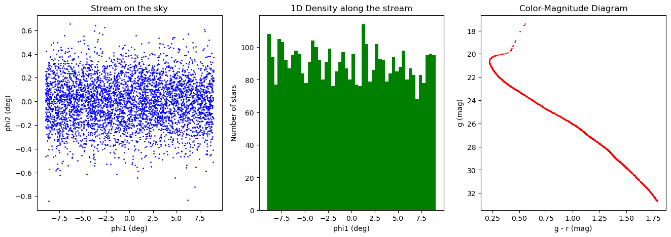
../_images/f339e0b73183cb3357ddb8a1c6292232e9d512e44a540bcbd39888570e8c8358.png

2) Spline-based configuration#

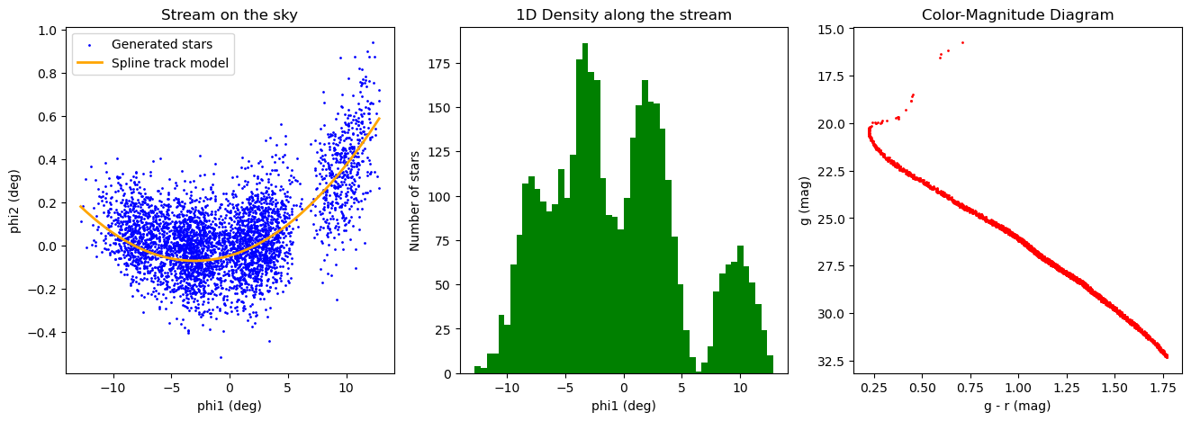
You can model a more realistic stream shape using cubic splines, particularly for:

Linear density: \(\sqrt{2\pi} \times \text{peak intensity} \times \text{spread}\)
Distance modulus
Track and width

In this example, we use data from data/patrick_2022_splines.csv and select stream == 'phoenix'.

# Nodes and values for the spline-based stream model (from Patrick et al. 2022, for Phoenix stream)
# One may read these from a CSV file instead of hardcoding them, cf to config/atlas_spline_config.yaml
intensity_nodes = np.array(
    [-13.0, -9.75, -8.125, -4.1640625, -3.25, -1.625, 1.625, 6.5, 8.125, 13.0]
)
intensity_node_values = np.array(
    [
        2.35582279e-07,
        2.65789495e-02,
        5.94765580e-02,
        7.20106921e-02,
        9.96003626e-02,
        4.68656926e-02,
        7.42352023e-02,
        4.75688845e-06,
        1.73046024e-02,
        4.08879937e-08,
    ]
)
spread_nodes = np.array([-13.0, 13.0])
spread_node_values = np.array([0.0992389, 0.17083177])
center_nodes = np.array([-13.0, 4.33333333, 13.0])
center_node_values = np.array([0.19313599, 0.07139282, 0.60245054])
distance_nodes = np.array([-13.0, 13.0])
distance_node_values = np.array([16.38285347, 16.1136374])


config_spline = {
    # Density model using cubic splines from CSV
    "density": {
        "type": "lineardensitycubicsplineinterpolation",
        "intensity_nodes": intensity_nodes,
        "intensity_node_values": intensity_node_values,
        "spread_nodes": spread_nodes,
        "spread_node_values": spread_node_values,
    },
    # Track model: center and spread as cubic splines
    "track": {
        "center": {
            "type": "CubicSplineInterpolation",
            "nodes": center_nodes,
            "node_values": center_node_values,
        },
        "spread": {
            "type": "CubicSplineInterpolation",
            "nodes": spread_nodes,
            "node_values": spread_node_values,
        },
    },
    # Isochrone model
    "isochrone": {
        "name": "Marigo2017",
        "survey": "lsst",
        "age": 13.0,
        "z": 0.0004,
        "band_1": "g",
        "band_2": "r",
        "band_1_detection": True,
    },
    # Distance modulus model as a cubic spline (flat default)
    "distance_modulus": {
        "center": {
            "type": "CubicSplineInterpolation",
            "nodes": distance_nodes,
            "node_values": distance_node_values,
        },
        "spread": {"type": "Constant", "value": 0.0},
    },
}

# Optional: sample using the spline-based config
stream_model_spline = StreamModel(config_spline)
stream_df_spline = stream_model_spline.sample(4000)

print(f"✓ Generated {len(stream_df_spline)} stars with spline density")
stream_df_spline.head()

✓ Generated 4000 stars with spline density

	phi1	phi2	dist	mu1	mu2	rv	lsst_g_true	lsst_r_true	mass
0	11.025280	0.206266	16.134085	None	None	None	27.764482	26.518739	0.189837
1	-3.956590	0.141461	16.289214	None	None	None	28.585344	27.239462	0.156199
2	11.894469	0.613266	16.125085	None	None	None	26.288612	25.246169	0.315157
3	-3.768348	-0.184497	16.287265	None	None	None	28.440219	27.112679	0.162797
4	3.090001	0.247316	16.216250	None	None	None	26.211489	25.189501	0.336810

fig, ax = plt.subplots(1, 3, figsize=(16, 5))

# plotting the stream on the sky
ax[0].scatter(
    stream_df_spline["phi1"],
    stream_df_spline["phi2"],
    s=1,
    color="blue",
    label="Generated stars",
)
x_val = np.sort(stream_df_spline["phi1"].values)
spline_val = scipy.interpolate.CubicSpline(center_nodes, center_node_values)(x_val)
ax[0].plot(x_val, spline_val, color="orange", lw=2, label="Spline track model")
ax[0].set_xlabel("phi1 (deg)")
ax[0].set_ylabel("phi2 (deg)")
ax[0].set_title("Stream on the sky")
ax[0].legend()

# Plotting the 1D density along the stream
ax[1].hist(stream_df_spline["phi1"], bins=50, color="green")
ax[1].set_xlabel("phi1 (deg)")
ax[1].set_ylabel("Number of stars")
ax[1].set_title("1D Density along the stream")

# plotting  Color magnitude diagram
ax[2].scatter(
    stream_df_spline["lsst_g_true"] - stream_df_spline["lsst_r_true"],
    stream_df_spline["lsst_g_true"],
    s=1,
    color="red",
)
ax[2].set_xlabel("g - r (mag)")
ax[2].set_ylabel("g (mag)")
ax[2].invert_yaxis()
ax[2].set_title("Color-Magnitude Diagram")

Text(0.5, 1.0, 'Color-Magnitude Diagram')

../_images/274d2f062f8702f40f6726f6f73c1d60a81dd1f35f893ab26c0b904950ad1c33.png

3) Complete an existing catalog#

StreamModel.complete_catalog fills only the requested columns while preserving existing values (except for magnitudes and velocities, which are regenerated together for consistency).

Dependencies:
- phi2 and dist require phi1
- mags require both dist and isochrone
Input formats: can be a DataFrame, dict, path to a CSV file, or None (with a specified size to generate the full catalog)

# Let's build a catalog with missing columns to complete
# Here for example we keep only 'phi1' and 'phi2', and drop others
stream_df_sub = stream_df.drop(
    columns=["lsst_r_true", "dist", "lsst_g_true", "mu1", "mu2", "rv"]
).reset_index(drop=True)
print("\nCatalog with missing columns:")
print(stream_df_sub.head())

Catalog with missing columns:
       phi1      phi2      mass
4.739512  0.015756  0.158219
-1.499554 -0.343139  0.246747
8.207016 -0.176948  0.387048
0.680482 -0.088033  0.299648
4.064195  0.077374  0.265148

Fill every missing columns#

# Now we can use `complete_catalog` to fill in the missing columns amoung ['phi1', 'phi2', 'dist', 'mag_g', 'mag_r', 'mu1', 'mu2', 'rv']
completed_catalog = stream_model.complete_catalog(
    catalog=stream_df_sub, save_path=None, inplace=False, verbose=True
)
print(completed_catalog.head())

Velocity model not defined; skipping velocities.
Filled 4500 dist values.
Filled ['lsst_g_true', 'lsst_r_true'] (missing rows only).
       phi1      phi2      mass  dist  lsst_g_true  lsst_r_true
0  4.739512  0.015756  0.158219  16.5    28.982359    27.582928
1 -1.499554 -0.343139  0.246747  16.5    27.581603    26.354772
2  8.207016 -0.176948  0.387048  16.5    26.265005    25.228614
3  0.680482 -0.088033  0.299648  16.5    27.004769    25.868177
4  4.064195  0.077374  0.265148  16.5    27.373922    26.179369

Fill only specific columns#

# Example: fill only magnitudes
subset = stream_df_sub.copy()
completed_mags = stream_model.complete_catalog(
    catalog=subset,
    columns_to_add=["lsst_g_true", "lsst_r_true"],
    inplace=False,
    verbose=True,
)
completed_mags.head()

Filled 4500 dist values.
Filled ['lsst_g_true', 'lsst_r_true'] (missing rows only).

	phi1	phi2	mass	dist	lsst_g_true	lsst_r_true
0	4.739512	0.015756	0.158219	16.5	28.982359	27.582928
1	-1.499554	-0.343139	0.246747	16.5	27.581603	26.354772
2	8.207016	-0.176948	0.387048	16.5	26.265005	25.228614
3	0.680482	-0.088033	0.299648	16.5	27.004769	25.868177
4	4.064195	0.077374	0.265148	16.5	27.373922	26.179369

Note: the distance modulus is also added, since it is needed to convert absolute magnitude sampled from the isochrone, to apparent magnitudes (mag_gand mag_r here).

Tips and Troubleshooting#

If magnitudes are missing or NaN, make sure your config includes both distance_modulus and isochrone sections.
To keep colors consistent, complete_catalog regenerates both mag_g and mag_r whenever one needs to be computed.
Column names are automatically standardized (e.g., 'g_mag' → 'mag_g'); see _standardize_columns_name.
The velocity model is currently a placeholder and returns NaN values.

Conclusion#

Streamobs provides a flexible framework to build and complete stellar stream mock catalogs, from simple analytic models to spline-based configurations. Future updates will include proper motions, velocities, and improved documentation for easier user adoption.

You can find more informations in the full documentation.

Streamobs: generate stream mocks

Contents