PWV effects on SN Magnitude¶

This notebook demonstrates the effects of PWV absorption on the apparent magnitude of SNe.

[1]:

import itertools
from copy import copy
from pathlib import Path

import numpy as np
from tqdm import tqdm

from matplotlib import pyplot as plt
from snat_sim import models, sn_magnitudes, plotting, constants as const
from tests.mock import create_mock_cadence

WARNING: AstropyDeprecationWarning: The update_default_config function is deprecated and may be removed in a future version. [sncosmo]

[2]:

fig_dir = Path('.') / 'figs' / 'delta_mag'
fig_dir.mkdir(exist_ok=True, parents=True)

We set some parameters for later use and create a Model that has a temporally static PWV transmission effect.

[3]:

model_without_pwv = models.SNModel('salt2-extended')
model_with_pwv = models.SNModel('salt2-extended')
model_with_pwv.add_effect(models.StaticPWVTrans(), '', 'obs')

pwv_vals = np.arange(0, 11)
z_vals = np.arange(.01, 1.05, .05)

# We make sure to use bands without an Atm. component
bands = [f'lsst_hardware_{b}' for b in 'grizy']

Spectral Template¶

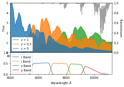
The effect of PWV absorption is fundamentally dependent on the interplay between the SED of the effected object and the PWV transmission function. For this work we consider an extend version of the Salt2 spectral template. We visualize the template as a reference. For easier visualization, the figure below includes dilation effects but does not include the change in flux density due to distance.

[4]:

_ = plotting.plot_spectral_template('salt2-extended', np.arange(4000, 10000), [0, .5, 1], pwv=4)
plt.savefig(fig_dir / 'spectral_template.pdf', bbox_inches='tight')

../_images/notebooks_sne_delta_mag_6_0.png

Apparent magnitude¶

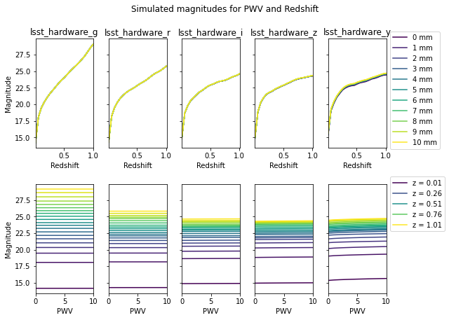
We start by considering the direct impact of PWV absorption on simulated SN Ia magnitudes. Apparent magnitudes are simulated for multiple bands, redshifts, and PWV concentrations.

[5]:

tabulated_mag = sn_magnitudes.tabulate_mag(model_with_pwv, pwv_vals, z_vals, bands)

Tabulating Mag: 100%|███████████████████████████████████████████████████████████████████████████████████████████████████████████████████████████████████████████████████████████████████████████████| 1155/1155 [00:02<00:00, 441.21it/s]

[6]:

fig, axes = plotting.plot_magnitude(tabulated_mag, pwv_vals, z_vals)
_ = fig.suptitle('Simulated magnitudes for PWV and Redshift', y=1.05)
plt.savefig(fig_dir / 'tabulated_magnitudes.pdf', bbox_inches='tight')

../_images/notebooks_sne_delta_mag_9_0.png

To better understand the impact of PWV, we estimate the change in apparent magnitude due to PWV. Although we could measure this change relative to PWV=0, a more physically motivated approach is to use a fiducial atmosphere with a non-zero PWV component:

\[\Delta m = m(\text{PWV}, z) - m(\text{PWV}_f, z)\]

We also determine the slope in the apparent magnitude as an estimate for how sensitive our simulated observations are to PWV fluctuations:

\[\frac{\Delta m}{\Delta \text{PWV}}(z) = \frac{m(\text{PWV}_2, z) - m(\text{PWV}_1, z)}{\text{PWV}_2 - \text{PWV}_1}\]

Here PWV\(_1\) and PWV\(_2\) are chosen to be equidistant to PWV\(_f\). We take note of the chosen PWV reference values in the following cell:

[7]:

reference_pwv_config = sn_magnitudes.get_config_pwv_vals()
print(reference_pwv_config)

{'reference_pwv': 4.0, 'slope_start': 2.0, 'slope_end': 6.0}

We tabulate values for \(\Delta m\) and \(\frac{\Delta m}{\Delta \text{PWV}}(z)\).

[8]:

tabulated_fiducial_mag = sn_magnitudes.tabulate_fiducial_mag(
        model_with_pwv, z_vals, bands, reference_pwv_config)

tabulated_delta_mag, tabulated_slope = sn_magnitudes.calc_delta_mag(
    tabulated_mag, tabulated_fiducial_mag, reference_pwv_config)

Tabulating Mag: 100%|█████████████████████████████████████████████████████████████████████████████████████████████████████████████████████████████████████████████████████████████████████████████████| 315/315 [00:00<00:00, 572.22it/s]

[9]:

fig, axes = plotting.plot_pwv_mag_effects(
    pwv_vals,
    z_vals,
    tabulated_delta_mag,
    tabulated_slope,
    bands)

_ = fig.suptitle('PWV Impact on Simulated magnitudes (Relative to Fiducial Atm.)', y=1.05)
plt.savefig(fig_dir / 'tabulated_pwv_effects.pdf', bbox_inches='tight')

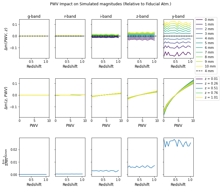
../_images/notebooks_sne_delta_mag_14_0.png

Sanity Check: We expect to see the following trends in the above plot: - The bluer bands should have minimal PWV impact. - The size of \(\Delta\)m should be largest for the redder bands. - The slope in \(\Delta\)m should be almost zero in the bluer bands. - \(\Delta\)m should be zero for the fiducial PWV value. - The general shape of the \(\Delta m\) vs PWV curves should change as a function of different features passing through each band. This means the shape of the curves should be different in each band.

Change in Magnitude With Fitting¶

Instead of tabulating the simulating magnitude, we can instead consider the change in magnitude by simulating light-curves with PWV effects and then fitting a model without a PWV component. For simplicity we use a densely sampled, uniform cadence.

[10]:

cadence = create_mock_cadence(bands=bands)
cadence

[10]:

<snat_sim.models.light_curve.ObservedCadence object at 0x7f49987b3460>
  time        band        gain  skynoise    zp   zpsys
------- --------------- ------- -------- ------- ------
  -20.0 lsst_hardware_g     1.0      0.0    30.0     AB
    ...             ...     ...      ...     ...    ...
   50.0 lsst_hardware_g     1.0      0.0    30.0     AB
   50.0 lsst_hardware_y     1.0      0.0    30.0     AB

[11]:

def iter_lcs_fixed_snr(cadence, model, pwv_arr, z_arr, snr = 10, verbose = True):
    """Iterator over SN light-curves for combination of PWV and z values

    Args:
        cadence (ObservedCadence): Observational cadence
        model           (SNModel): The sncosmo model to use in the simulations
        pwv_arr        (np.array): Array of PWV values
        z_arr          (np.array): Array of redshift values
        snr          (float, int): Signal to noise ratio
        verbose            (bool): Show a progress bar

    Yields:
        An Astropy table for each PWV and redshift
    """

    model = copy(model)
    iter_total = len(pwv_arr) * len(z_arr)
    arg_iter = itertools.product(pwv_arr, z_arr)
    for pwv, z in tqdm(arg_iter, total=iter_total, desc='Light-Curves', disable=not verbose):
        # Update model to reflect the parameters we want to use in the simulation
        model.set(t0=0.0, pwv=pwv, z=z)
        model.set_source_peakabsmag(const.betoule_abs_mb, 'standard::b', 'AB', cosmo=const.betoule_cosmo)

        # Simulate a light-curve and convert it from a ``LightCurve`` instance to an astropy table
        light_curve = model.simulate_lc(cadence, scatter=False, fixed_snr=snr).to_astropy()
        light_curve.meta = dict(zip(model.param_names, model.parameters))

        yield light_curve

[12]:

# Fit light curves
vparams = ['x0', 'x1', 'c']
light_curves = iter_lcs_fixed_snr(cadence, model_with_pwv, pwv_vals, z_vals)

fitted_mag, fitted_params = sn_magnitudes.fit_mag(
    model_without_pwv,
    light_curves,
    vparams,
    bands,
    pwv_vals,
    z_vals)

Light-Curves: 100%|████████████████████████████████████████████████████████████████████████████████████████████████████████████████████████████████████████████████████████████████████████████████████| 231/231 [03:18<00:00,  1.16it/s]

[13]:

# Fit light curves at reference PWV vals
reference_pwv_vals = [reference_pwv_config['slope_start'], reference_pwv_config['reference_pwv'], reference_pwv_config['slope_end']]
reference_light_curves = iter_lcs_fixed_snr(cadence, model_with_pwv, reference_pwv_vals, z_vals)

# Get fiducial mag
fitted_fiducial_mag, fitted_fiducial_params = sn_magnitudes.fit_mag(
    model_without_pwv,
    reference_light_curves,
    vparams,
    bands,
    reference_pwv_vals,
    z_vals)

Light-Curves: 100%|██████████████████████████████████████████████████████████████████████████████████████████████████████████████████████████████████████████████████████████████████████████████████████| 63/63 [00:54<00:00,  1.16it/s]

Here we visualize the fitted, uncorrected (i.e. without any stretch / color correction) magnitudes.

[14]:

fig, axes = plotting.plot_magnitude(fitted_mag, pwv_vals, z_vals)
_ = fig.suptitle('Fitted Magnitude (Uncorrected)', y=1.05)
plt.savefig(fig_dir / 'fitted_magnitudes.pdf', bbox_inches='tight')

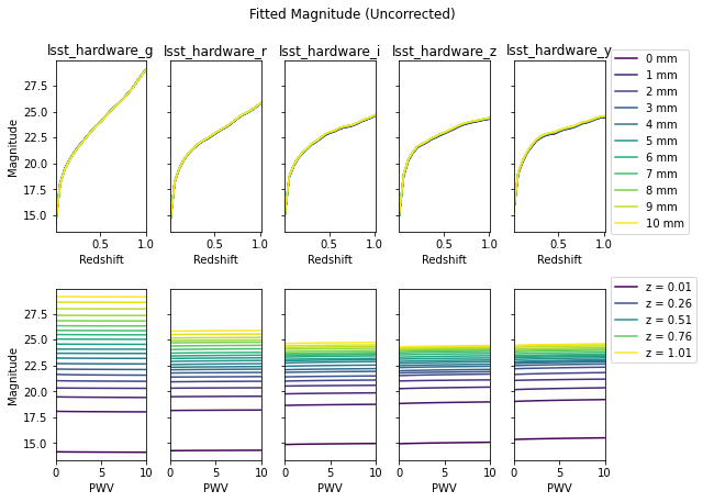
../_images/notebooks_sne_delta_mag_22_0.png

Sanity Check: The fitted light-curves are constructed to have a dense, uniform sampling. As a result, the fitted magnitude should look extremely similar to the tabulated magnitudes from earlier.

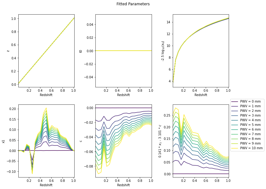
We expect to see minimal differences between the tabulated, and fitted magnitudes in each band. However, we do expect to variation in the fitted stretch and color.

[15]:

fig, axes = plotting.plot_fitted_params(fitted_params, pwv_vals, z_vals, bands)
_ = fig.suptitle('Fitted Parameters', y=1.05)
plt.savefig(fig_dir / 'fitted_parameters.pdf', bbox_inches='tight')

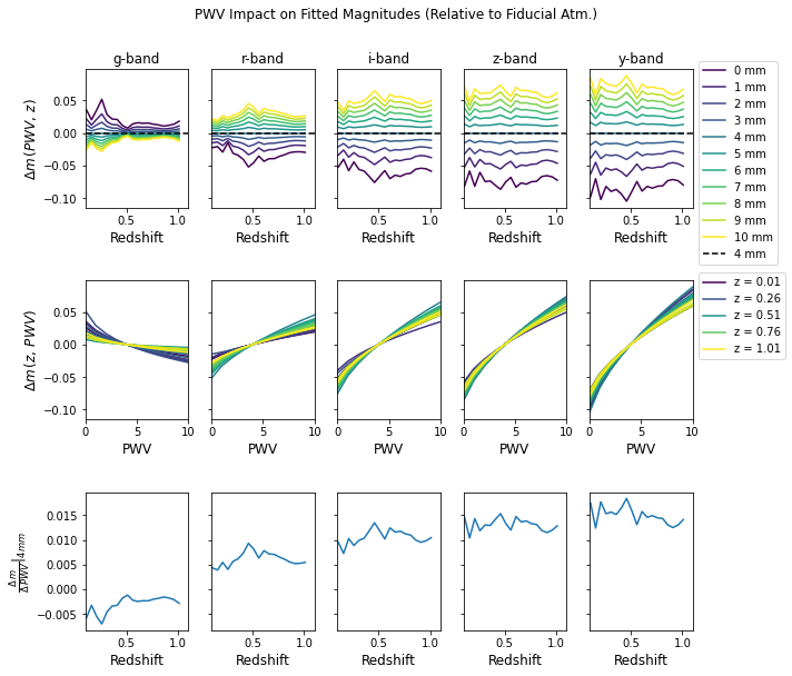
../_images/notebooks_sne_delta_mag_25_0.png

We look at the impact of PWV on the fitted magnitude.

[16]:

corrected_delta_mag, corrected_slope = sn_magnitudes.calc_delta_mag(
    fitted_mag, fitted_fiducial_mag, reference_pwv_config)

[17]:

fig, axes = plotting.plot_pwv_mag_effects(
    pwv_vals,
    z_vals,
    corrected_delta_mag,
    corrected_slope,
    bands)

_ = fig.suptitle('PWV Impact on Fitted Magnitudes (Relative to Fiducial Atm.)', y=1.05)
plt.savefig(fig_dir / 'fitted_pwv_effects.pdf', bbox_inches='tight')

../_images/notebooks_sne_delta_mag_28_0.png

Next we add in the alpha and beta parameters from the fit.

[18]:

# Determine corrected magnitude from fits
corrected_mag = {}
corrected_fiducial_mag = {}
for band in bands:
    corrected_mag[band] = sn_magnitudes.correct_mag(
        model_with_pwv, fitted_mag[band], fitted_params[band])

    # Get fiducial mag (calibrated)
    corrected_fiducial_mag[band] = sn_magnitudes.correct_mag(
        model_with_pwv, fitted_fiducial_mag[band], fitted_fiducial_params[band])

[19]:

corrected_delta_mag, corrected_slope = sn_magnitudes.calc_delta_mag(
        corrected_mag, corrected_fiducial_mag, reference_pwv_config)

[20]:

fig, axes = plotting.plot_pwv_mag_effects(
    pwv_vals,
    z_vals,
    corrected_delta_mag,
    corrected_slope,
    bands)

_ = fig.suptitle('PWV Impact on Calibrated Magnitudes (Relative to Fiducial Atm.)', y=1.05)
plt.savefig(fig_dir / 'corr_pwv_effects.pdf', bbox_inches='tight')

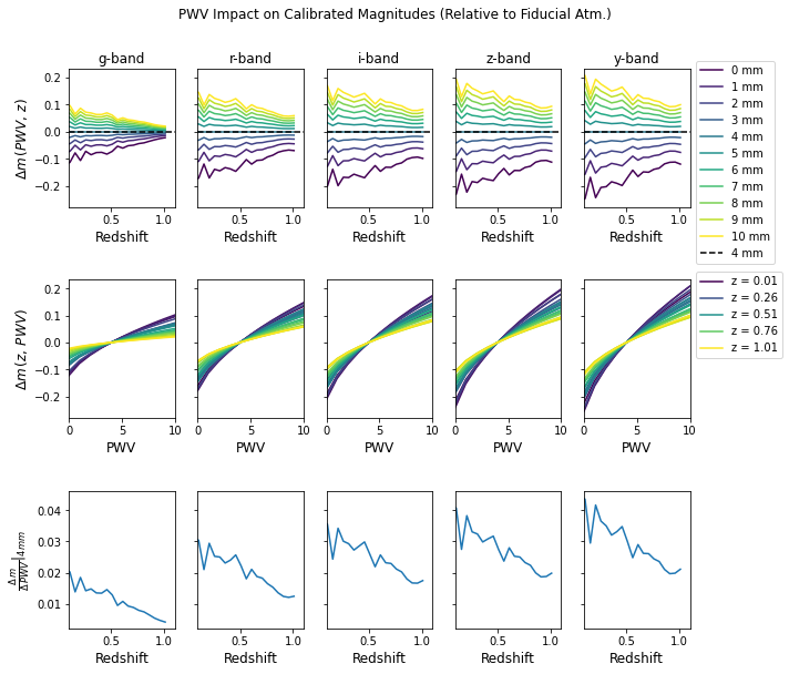
../_images/notebooks_sne_delta_mag_32_0.png

Sanity Check: Unlike some of the previous plots we have made, we expect the overall shape of the the \(\Delta m\) vs \(z\) curves to be similar across bands. Since we are considering fitted magnitudes in the above plot, the presence of PWV impacts the fitted model parameters, and then the model enforces cross-band uniformity when we evaluate the synthetic photometry.

Relative to a Reference Star¶

In practice flux values are calibrated relative to a reference star. To understand how PWV effects SNe fluxes during this process, we normalize the reference star flux to it’s respective fluxes through PWV=0 and take the difference (SNe flux / normalized reference star flux).

[21]:

def iter_light_curves_with_ref(model, pwv_arr, z_arr, spectral_types=('G2', 'M5', 'K2'), snr = 10, verbose = True):
    """Iterator over SN light-curves calibrated to a set of reference stars

    Args:
        model            (SNModel): The sncosmo model to use in the simulations
        pwv_arr         (np.array): Array of PWV values
        z_arr           (np.array): Array of redshift values
        spectral_types (list[str]): Spectral types to use in the calibration
        snr           (float, int): Signal to noise ratio
        verbose             (bool): Show a progress bar

    Yields:
        An Astropy table for each PWV and redshift
    """

    catalog = models.ReferenceCatalog(*spectral_types)
    for lc in iter_lcs_fixed_snr(cadence, model, pwv_arr, z_arr, snr=snr, verbose=verbose):
        pwv = lc.meta['pwv']
        new_lc = catalog.calibrate_lc(models.LightCurve.from_sncosmo(lc), pwv=pwv).to_astropy()
        new_lc.meta = lc.meta
        yield new_lc

[22]:

vparams = ['x0', 'x1', 'c']
light_curves_with_ref = iter_light_curves_with_ref(model_with_pwv, pwv_vals, z_vals)
fitted_mag_with_ref, fitted_params_with_ref = sn_magnitudes.fit_mag(
        model_without_pwv, light_curves_with_ref, vparams, bands, pwv_vals, z_vals, bounds={'t0': (-1, 1)})

Light-Curves: 100%|████████████████████████████████████████████████████████████████████████████████████████████████████████████████████████████████████████████████████████████████████████████████████| 231/231 [03:10<00:00,  1.21it/s]

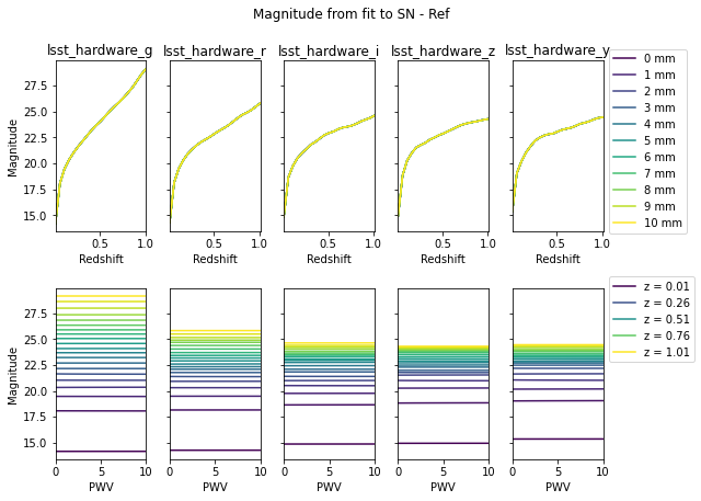
[23]:

fig, axes = plotting.plot_magnitude(fitted_mag_with_ref, pwv_vals, z_vals)
_ = fig.suptitle('Magnitude from fit to SN - Ref', y=1.05)

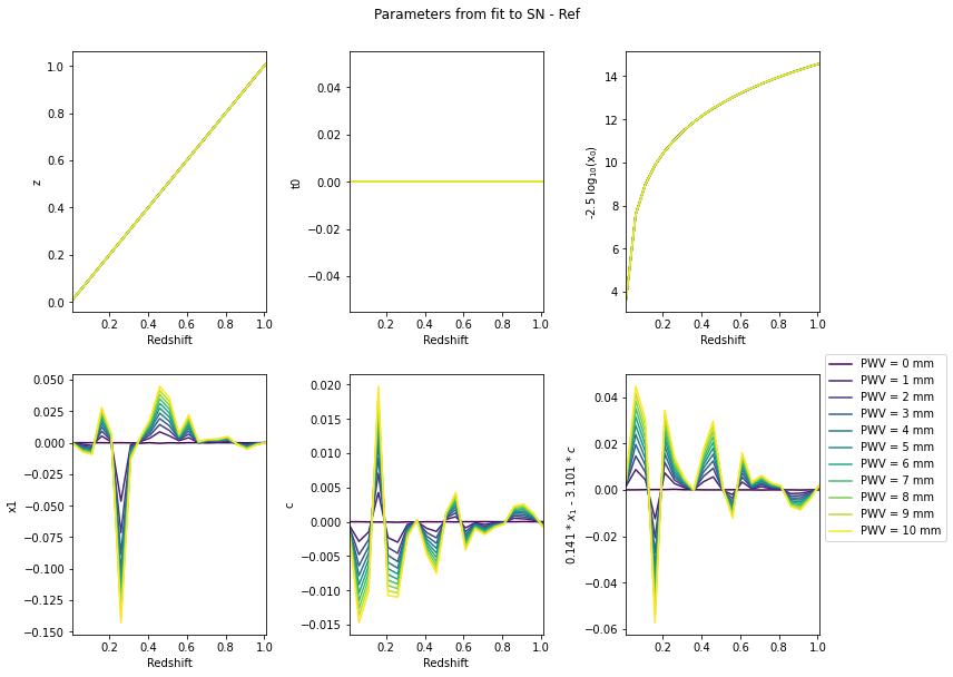
../_images/notebooks_sne_delta_mag_38_0.png

[24]:

fig, axes = plotting.plot_fitted_params(fitted_params_with_ref, pwv_vals, z_vals, bands)
_ = fig.suptitle('Parameters from fit to SN - Ref', y=1.05)

../_images/notebooks_sne_delta_mag_39_0.png

[25]:

# Determine corrected magnitude from fits
corrected_mag_with_ref = {}
for band in bands:
    corrected_mag_with_ref[band] = sn_magnitudes.correct_mag(
        model_with_pwv, fitted_mag_with_ref[band], fitted_params_with_ref[band])

[26]:

fig, axes = plotting.plot_magnitude(corrected_mag_with_ref, pwv_vals, z_vals)
_ = fig.suptitle('Corrected Magnitude from fit to SN - Ref', y=1.05)

../_images/notebooks_sne_delta_mag_41_0.png

[27]:

_pwv_list = list(pwv_vals)
reference_idx = _pwv_list.index(reference_pwv_config['reference_pwv'])
slope_start_idx = _pwv_list.index(reference_pwv_config['slope_start'])
slope_end_idx = _pwv_list.index(reference_pwv_config['slope_end'])

corrected_fiducial_mag_with_ref = dict()
for band in bands:
    _mag_arr = corrected_mag_with_ref[band]
    _ref_mag = _mag_arr[reference_idx]
    _start_mag = _mag_arr[slope_start_idx]
    _end_mag = _mag_arr[slope_end_idx]

    corrected_fiducial_mag_with_ref[band] = [_start_mag, _ref_mag, _end_mag]

[28]:

corrected_delta_mag_with_ref, corrected_slope_with_ref = sn_magnitudes.calc_delta_mag(
        corrected_mag_with_ref, corrected_fiducial_mag_with_ref, reference_pwv_config)

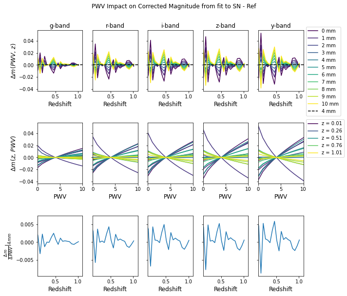
fig, axes = plotting.plot_pwv_mag_effects(
    pwv_vals,
    z_vals,
    corrected_delta_mag_with_ref,
    corrected_slope_with_ref,
    bands)

fig.suptitle('PWV Impact on Corrected Magnitude from fit to SN - Ref', y=1.05)
plt.savefig(fig_dir / 'corr_pwv_effects_with_ref_star.pdf', bbox_inches='tight')

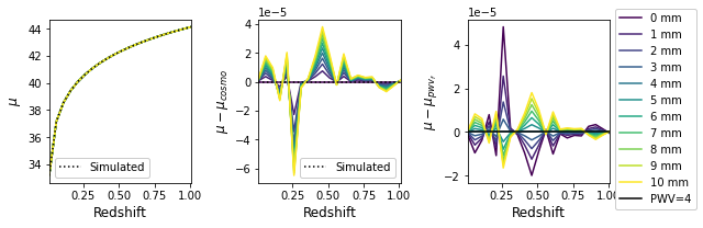
../_images/notebooks_sne_delta_mag_43_0.png

Impact on Distance Modulus¶

Here we consider the impact of PWV on \(\mu\) using fits to SNe flux after calibration to the reference star. We note that there is a disagreement between the distance module calculated by an astropy Cosmology object, and by an SNCosmo model that has been calibrated using that same cosmology. For consistency, we exclusively use SNCosmo values of \(\mu\).

Results without using a reference star¶

[29]:

# The params are band independent so we use the r-band values
calib_factor = sn_magnitudes.calc_calibration_factor_for_params(
    model_without_pwv, fitted_params['lsst_hardware_r'])

fitted_mu = sn_magnitudes.calc_mu_for_params(
    model_without_pwv, fitted_params['lsst_hardware_r'])

[30]:

# Account for (what I think is) a numerical error between astropy and sncosmo
numerical_error_offset = fitted_mu[0] - const.betoule_cosmo.distmod(z_vals).value

plotting.plot_delta_mu(fitted_mu - numerical_error_offset, pwv_vals, z_vals)

../_images/notebooks_sne_delta_mag_47_0.png

[31]:

plotting.plot_delta_mu(fitted_mu + calib_factor - numerical_error_offset, pwv_vals, z_vals)
plt.savefig(fig_dir / 'mu_pwv_effects.pdf', bbox_inches='tight')

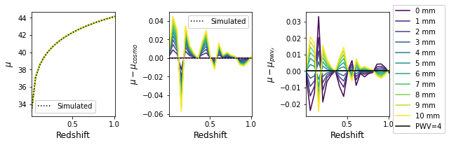
../_images/notebooks_sne_delta_mag_48_0.png

Results with a reference star¶

[32]:

calib_factor_with_ref = sn_magnitudes.calc_calibration_factor_for_params(
    model_without_pwv, fitted_params_with_ref['lsst_hardware_r'])

fitted_mu_with_ref = sn_magnitudes.calc_mu_for_params(
    model_without_pwv, fitted_params_with_ref['lsst_hardware_r'])

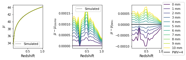
[33]:

numerical_error_offset_ref = fitted_mu_with_ref[0] - const.betoule_cosmo.distmod(z_vals).value
plotting.plot_delta_mu(fitted_mu_with_ref - numerical_error_offset_ref, pwv_vals, z_vals)

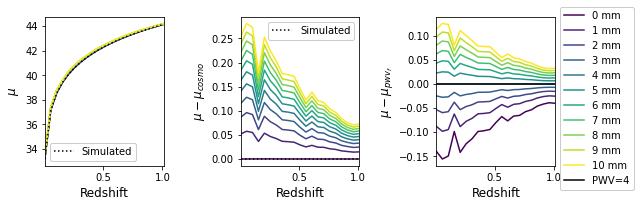
../_images/notebooks_sne_delta_mag_51_0.png

[34]:

plotting.plot_delta_mu(fitted_mu_with_ref + calib_factor_with_ref - numerical_error_offset_ref, pwv_vals, z_vals)
plt.savefig(fig_dir / 'mu_pwv_effects_with_ref.pdf', bbox_inches='tight')

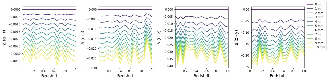
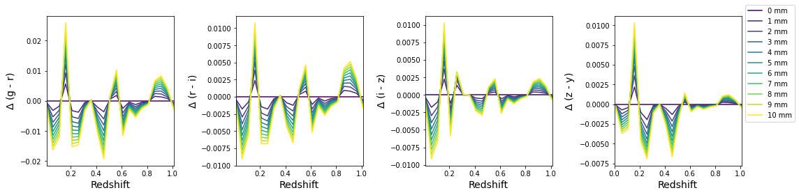
../_images/notebooks_sne_delta_mag_52_0.png

Change in Color¶

[35]:

colors = list(zip(bands[:-1], bands[1:]))

[36]:

plotting.plot_delta_colors(pwv_vals, z_vals, tabulated_mag, colors)
plt.savefig(fig_dir / 'delta_tabulated_corrected_color.pdf', bbox_inches='tight')

../_images/notebooks_sne_delta_mag_55_0.png

[37]:

plotting.plot_delta_colors(pwv_vals, z_vals, corrected_mag, colors)
plt.savefig(fig_dir / 'delta_fitted_corrected_color.pdf', bbox_inches='tight')

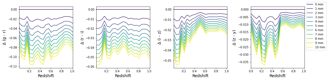
../_images/notebooks_sne_delta_mag_56_0.png

[38]:

plotting.plot_delta_colors(pwv_vals, z_vals, corrected_mag_with_ref, colors)
plt.savefig(fig_dir / 'delta_fitted_color_with_ref.pdf', bbox_inches='tight')

../_images/notebooks_sne_delta_mag_57_0.png

[ ]:

Table Of Contents