Machine Learning

We showed earlier that a single color measurement can be used to help predict chromatic biases. A natural next step is to see what additional information is contained in the remaining four LSST photometric data points.

The scripts star_ML.py and gal_ML.py in the bin/analytic/catalogs/ directory are used for this purpose. These scripts will apply a machine learning algorithm – Support Vector Regression – to learn the relationship in a catalog between LSST six-band photometry and chromatic biases. (Other machine learning algorithms can easily be swapped in by modifying the scripts: the scikit-learn API is quite flexible.)

Let’s look at the options for the star_ML.py script.

$ cd CHROMA_DIR/bin/analytic/catalog/
$ python star_ML.py --help
usage: star_ML.py [-h] [--trainfile TRAINFILE] [--testfile TESTFILE]
                  [--outfile OUTFILE] [--trainstart TRAINSTART]
                  [--ntrain NTRAIN] [--teststart TESTSTART] [--ntest NTEST]
                  [--use_color] [--use_mag]

optional arguments:
  -h, --help            show this help message and exit
  --trainfile TRAINFILE
                        file containing training data (Default:
                        output/star_data.pkl)
  --testfile TESTFILE   file containing testing data (Default:
                        output/star_data.pkl)
  --outfile OUTFILE     output file (Default: output/corrected_star_data.pkl)
  --trainstart TRAINSTART
                        object index at which to start training (Default: 0)
  --ntrain NTRAIN       number of objects on which to train ML (Default:
                        16000)
  --teststart TESTSTART
                        object index at which to start training (Default:
                        16000)
  --ntest NTEST         number of objects on which to test ML (Default: 4000)
  --use_color           use only colors as features (Default: colors + 1
                        magnitude)
  --use_mag             use only magnitudes as features (Default: colors + 1
                        magnitude)

By default, the output/star_data.pkl file which we either created or downloaded on the previous pages is used for both training the algorithm and testing it. In principle, however, you can train on one set of data and test on another set, which can be useful for estimating the robustness of the algorithm to uncertainties in the distribution of training objects. I.e., you can train an one catalog, and then see if the results are still useful for predicting the biases in a completely different catalog. Several more options control which and how many stars are used for testing and training.

The objects in the testing set are written to an output file which contains both the true spectroscopically-derived chromatic biases, and the chromatic biases predicted from photometry by the machine learning algorithm.

Finally, there are two options that control how the photometric data is used. The --use_color option trains the SVR algorithm to predict chromatic biases from just the 5 independent LSST colors. In contrast, the --use_mag option trains from the 6 LSST magnitudes directly. We have found the best results in practice occur, however, when we train the algorithm using the 5 independent colors + 1 independent magnitude (arbitrarily chosen to be $i$ band); this is the default.

For now, let’s just proceed with the default options. (Note that these scripts take ~30-45 minutes each on a 2012 Macbook Pro).

$ python star_ML.py
$ python gal_ML.py
$ ls output/corrected*
output/corrected_galaxy_data.pkl  output/corrected_star_data.pkl

We can use the same script as on the previous page to plot the results: plot_bias.py. This time, we don’t even need to specify --starfile and --galfile, since the defaults will work just fine. Additionally, we can now go ahead and use the --corrected flag to plot not the relative chromatic biases between different stars and galaxies, but the residual chromatic biases from the photometric estimates. Let’s use the --nominal_plots flag again to quickly make the most interesting plots.

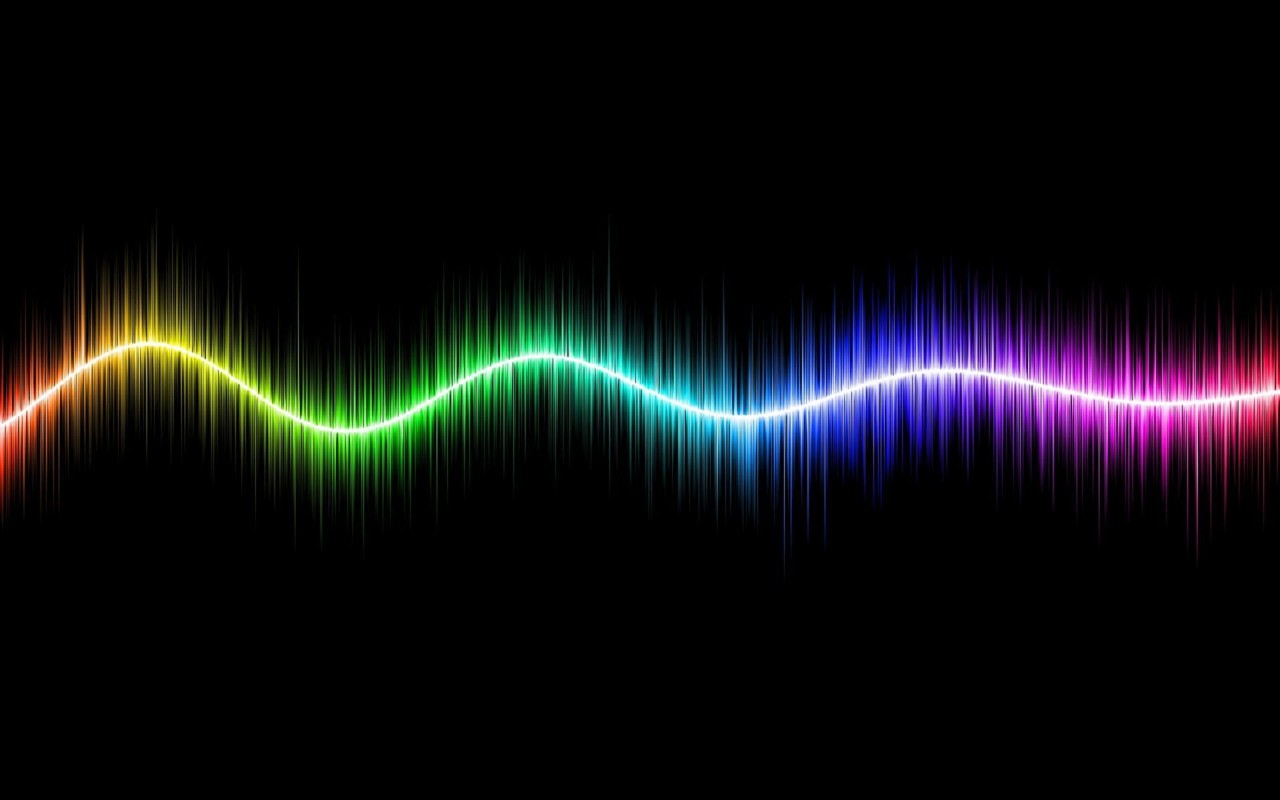
$ python plot_bias.py --corrected --nominal_plots

You can mouseover the following plots to see the uncorrected versions. (Note that these plots are slightly different the ones on the previous page. They’ve been regenerated to use precisely the same galaxies as the corrected versions, i.e. they use only the galaxies from the test set.)

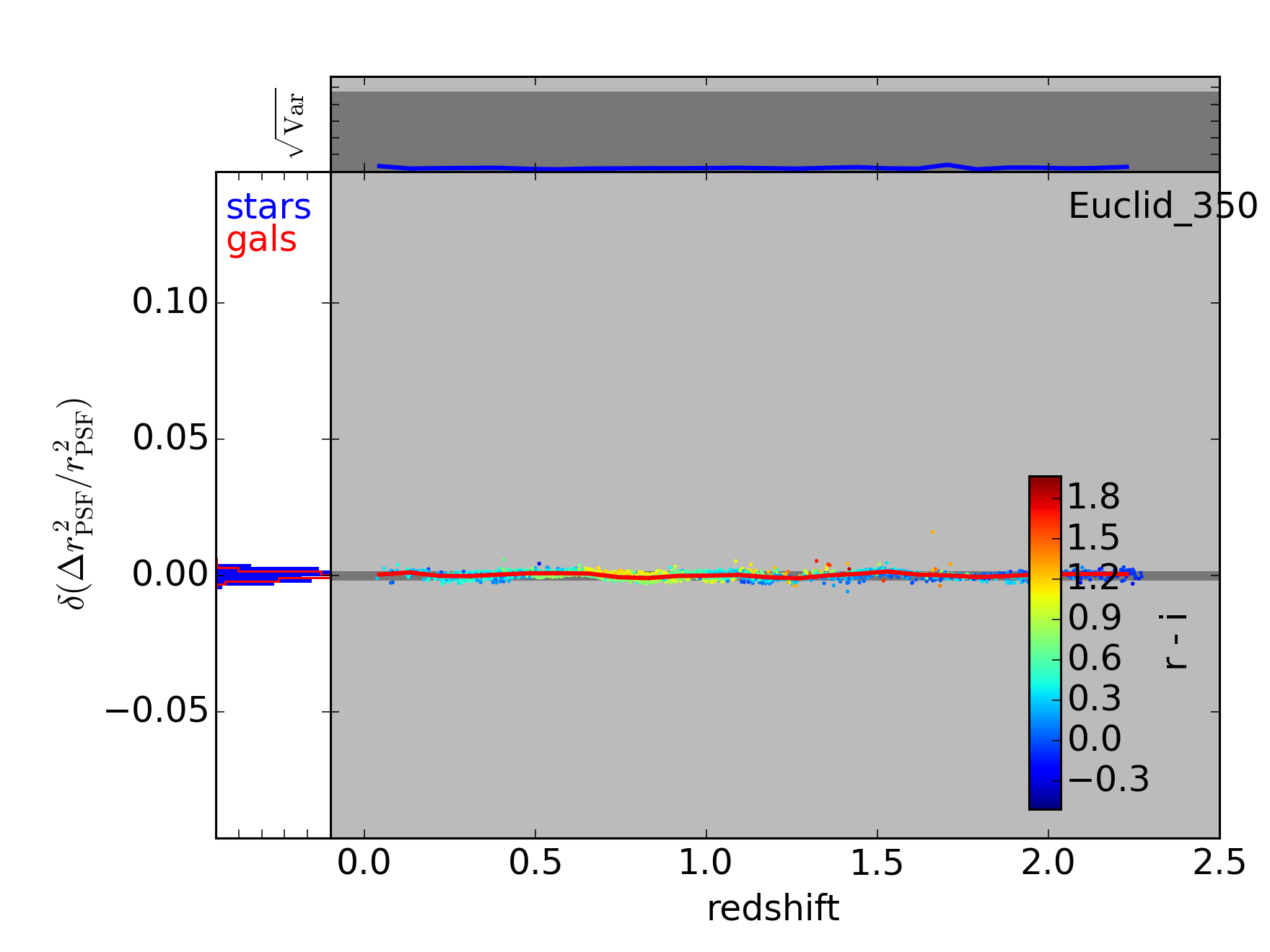
In this last figure, we’re using LSST photometry to help correct the Euclid chromatic bias. This correction does a particularly good job since the Euclid 350nm visible filter is approximately the union of the LSST $r$ , $i$ , and $z$ filters. These three LSST filters provide quite of bit of information, therefore, as to what the SED of a star or galaxy looks like across the Euclid filter. Note that the LSST sky overlaps the proposed Euclid sky by about 5000 square degrees, or about a third of either survey’s footprint.

Back