Catalog Results

The previous pages looked at chromatic biases that arise for a set of standard template stellar and galactic SEDs. In the real Universe, the distribution of SEDs is much more complicated. Here we take a look at the distribution of chromatic biases for a more realistic set of SEDs obtained from the LSST catalog framework.

We provide two methods for users to obtain a realistic catalog of stellar and galactic magnitudes and chromatic biases. The software to produce such a catalog using the LSST Image Simulation catalog framework is included in Chroma, and its use is detailed below. The catalog framework can be a bit tricky to work with, however, and requires downloading a large collection (~3.5 Gb) of unreddened rest-frame SEDs. As an alternative, we also provide the resulting catalogs of magnitudes and biases as a separate download.

Making the chromatic bias catalogs

The first catalog script we’ll look at is make_catalogs.py. This is the only script in Chroma that requires the LSST catalog framework to run. It queries the LSST catalog simulation (CatSim) database for stars and galaxies inside a 1 degree patch. The stars are selected to have i band magnitude between 16 and 22, which is approximately the range useable for PSF estimation. The galaxies are selected to be brighter than i < 25.3, which is referred to as the LSST “gold sample” for weak lensing. These are galaxies that should yield reasonable signal-to-noise for shape estimates. The returned catalog entries are written to the files output/galaxy_catalog.dat and output/star_catalog.dat.

$ cd CHROMA_DIR/bin/analytic/catalog/
$ python make_catalogs.py
$ ls output/
output/galaxy_catalog.dat
output/star_catalog.dat

Note that access to the LSST CatSim database now requires your IP address to be on a white list.

Let’s take a look at the galaxy catalog file

$ head -n 3 output/galaxy_catalog.dat
galtileid, objectId, raJ2000, decJ2000, redshift, u_ab, g_ab, r_ab, i_ab, z_ab, y_ab, sedPathBulge, sedPathDisk, sedPathAgn, magNormBulge, magNormDisk, magNormAgn, internalAvBulge, internalRvBulge, internalAvDisk, internalRvDisk, glon, glat, EBV
222500350435, 222500350435, 199.56648010, -9.28911042, 0.87100780, 24.72078514, 24.37876129, 23.35155296, 22.37948418, 21.74126053, 21.46795082, galaxySED/Burst.32E09.02Z.spec.gz, galaxySED/Exp.40E09.04Z.spec.gz, None, 25.08109093, 21.86528015, nan, 0.30000001, 3.09999990, 0.40000001, 3.09999990, 5.47990054, 0.92513679, 0.03601249
222501392641, 222501392641, 199.57937323, -9.29996667, 0.70250392, 26.08153725, 25.31512642, 24.57574654, 23.79152298, 23.51052094, 23.27629852, galaxySED/Inst.50E09.04Z.spec.gz, galaxySED/Const.50E09.04Z.spec.gz, None, 26.84174919, 23.30666924, nan, 0.10000000, 3.09999990, 0.80000001, 3.09999990, 5.48020956, 0.92491178, 0.03617451

The first line shows the names of each database column requested in make_catalogs.py, and each subsequent line holds the values for one galaxy. The columns are:

galtileid, objectID : These keep track of which galaxy we’re looking at
raJ2000, decJ2000, redshift : Where the galaxy is located (in 3D)
u_ab - y_ab : AB magnitudes through the LSST ugrizy filters.
sedPathBulge : Name of the rest-frame unreddened SED file representing the bulge component of the galaxy.
magNormBulge : The AB magnitude of the bulge component at 500nm rest-frame
internalAvBulge, internalRvBulge : The rest frame reddening of the bulge component
similar params for the disk component and possible AGN component
galactic latitude and longitude and Milky Way dust E(B-V)

The stellar catalog has similar entries, although somewhat simpler since the stars are single component.

Our goal is to take these parameters, construct the observed frame SED (including bulge, disk, and AGN components, dust, and redshift), and calculate the relative chromatic biases for each star and galaxy. This is precisely what the scripts process_gal_catalog.py and process_star_catalog.py do. Users may in particular wish to look at the functions process_gal_catalog.py:composite_spectrum() and process_star_catalog.py:stellar_spectrum() to see exactly how the observed frame SEDs are generated. The output of the processing scripts are pickle files containing catalog and synthetic photometry, and calculated chromatic biases.

$ python process_gal_catalog.py
$ python process_star_catalog.py
$ ls output/*.pkl
output/galaxy_data.pkl
output/star_data.pkl

Download chromatic biases catalogs

Since the LSST catalog framework can be somewhat tricky to install, we have also made the catalog files that would be created by process_gal_catalog.py and process_star_catalog.py available online. You can download the files with a web browser and place them in the bin/analytic/catalog/output/ directory or use a utility like curl:

$ cd DIRECTORY_TO_CHROMA/bin/analytic/catalog/output/
$ ls
$ curl -O slac.stanford.edu/~jmeyers3/galaxy_data.pkl
$ curl -O slac.stanford.edu/~jmeyers3/star_data.pkl
$ ls
galaxy_data.pkl
star_data.pkl

Plots

With the processed catalog data in place, we can look at the distribution of chromatic biases for a realistic population of lensing galaxies. The tool for generating catalog bias plots is plot_bias.py. This script takes a number of command-line options, which can be listed with the --help option:

$ python plot_bias.py --help
usage: plot_bias.py [-h] [--galfile GALFILE] [--starfile STARFILE]
                    [--corrected] [--band [BAND]] [--color COLOR COLOR]
                    [--outfile [OUTFILE]] [--nominal_plots]
                    [bias]

positional arguments:
  bias                 which chromatic bias to plot (Default: 'Rbar') Other
                       possibilities include: 'V', 'S_m02', 'S_p06', 'S_p10'

optional arguments:
  -h, --help           show this help message and exit
  --galfile GALFILE    input galaxy file. Default
                       'output/corrected_galaxy_data.pkl'
  --starfile STARFILE  input star file. Default
                       'output/corrected_star_data.pkl'
  --corrected          plot learning residuals instead of G5v residuals.
  --band [BAND]        band of chromatic bias to plot (Default: 'LSST_r')
  --color COLOR COLOR  color to use for symbol color (Default: ['LSST_r',
                       'LSST_i'])
  --outfile [OUTFILE]  output filename (Default: 'output/chromatic_bias.png')
  --nominal_plots      Plot some nominal useful LSST and Euclid figures

Notice that the default input files: output/corrected_galaxy_data.pkl and output/corrected_star_data.pkl don’t exist yet. This is because these are the files that will be created under the machine learning corrections step on the next page. For now we can use the uncorrected catalog files by adding them manually as command line arguments. For instance, to make a plot of the squared centroid shift bias with a logarithmic axis in the r band due to DCR, use:

$ python plot_bias.py LnRbarSqr --galfile output/galaxy_data.pkl \
                                --starfile output/star_data.pkl  \
                                --outfile output/dLnRbarSqr.LSST_r.png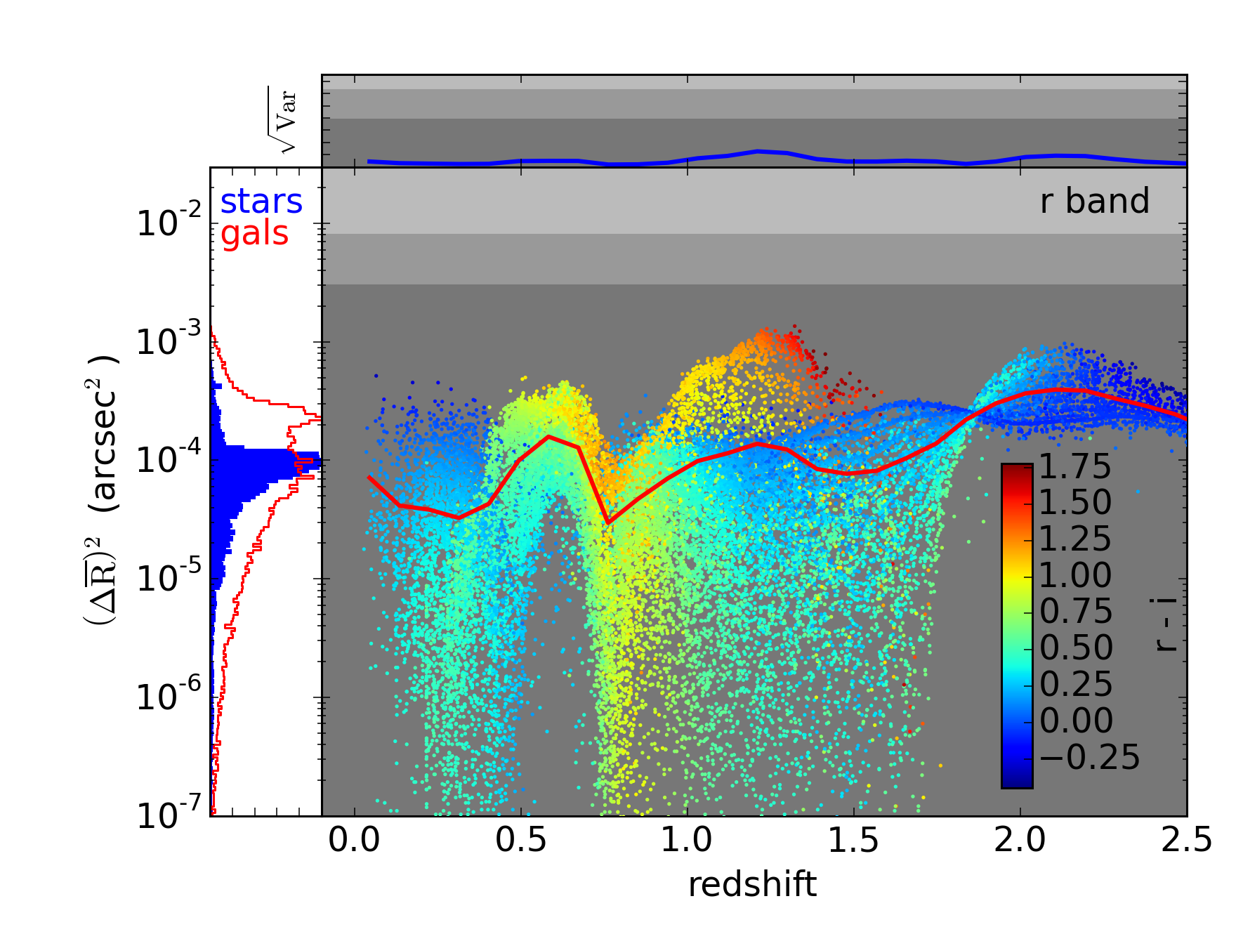

Each point of the scatter plot is one galaxy from the catalog. The points are colored by their $r$ - $i$ color, with both very blue and very red objects having large squared centroid shifts. The histograms on the left show the distributions of squared centroid shifts for stars in blue, and the galaxies projected along the redshift axis in red. The dark horizontal bars again show the requirements for DES and LSST.

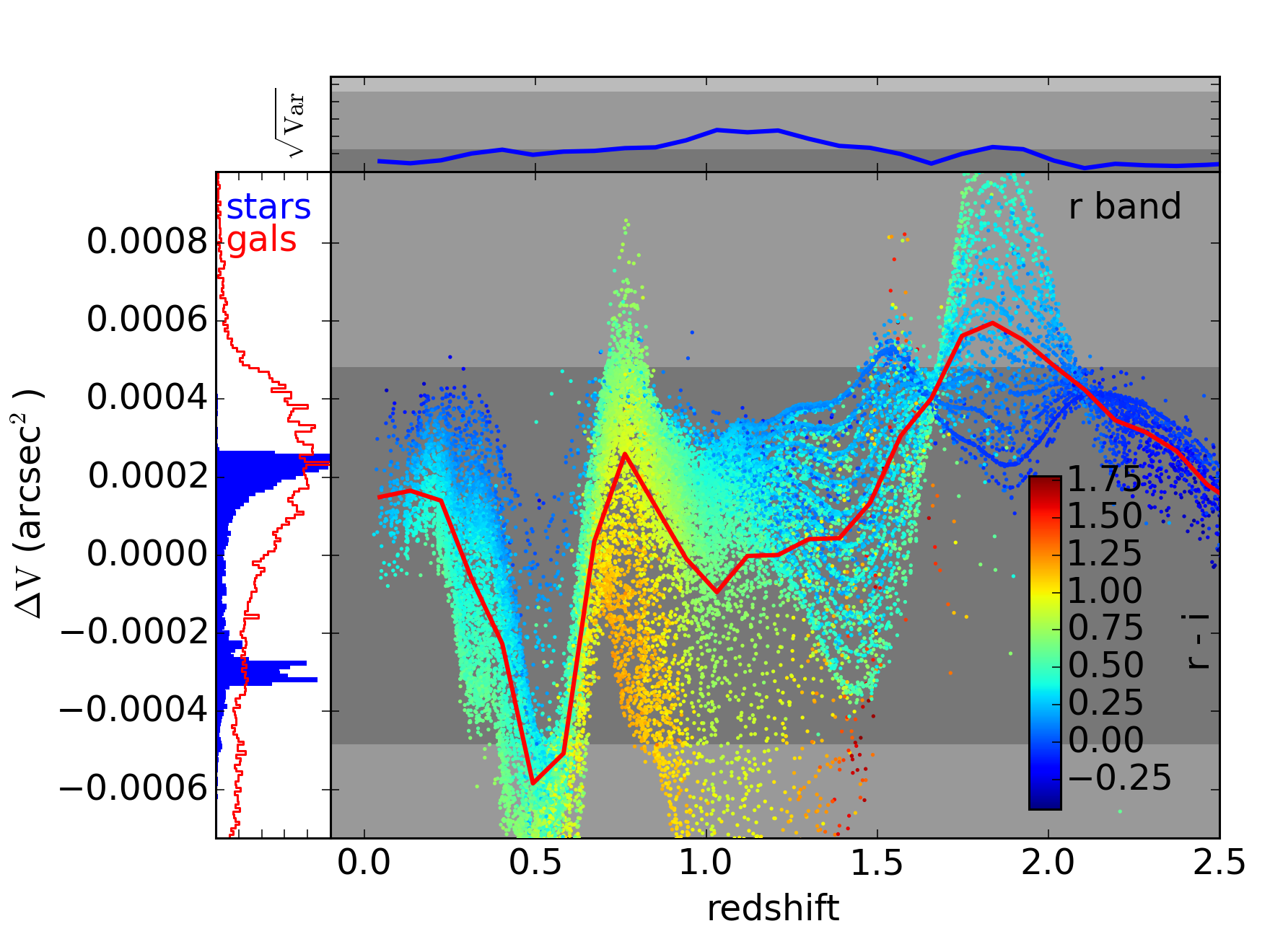
To quickly plot a number of interesting plots, we can use plot_bias.py with the option --nominal_plots.

$ python plot_bias.py --galfile output/galaxy_data.pkl \
                      --starfile output/star_data.pkl \
                      --nominal_plots

Here are a few of the more interesting cases.

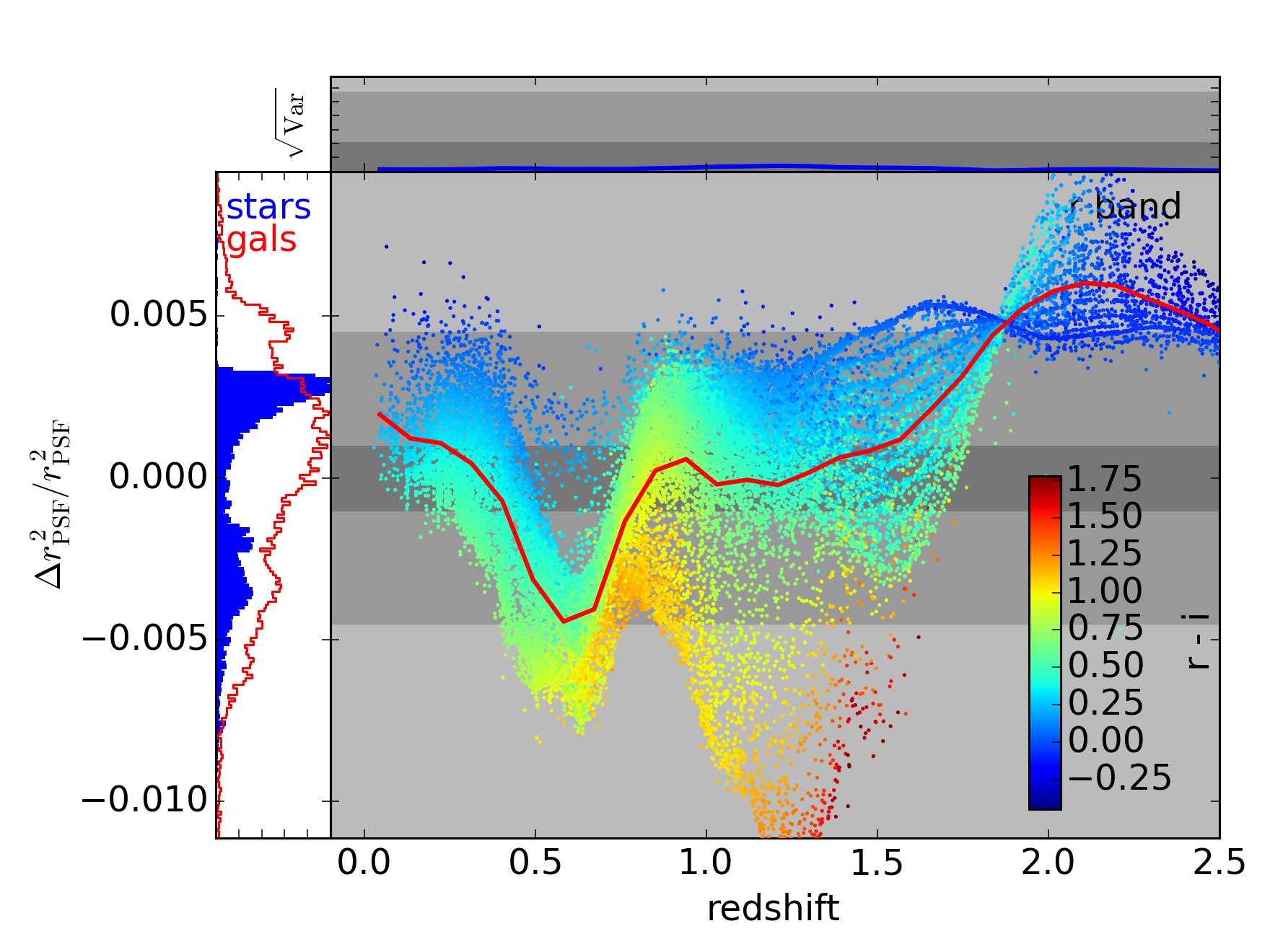
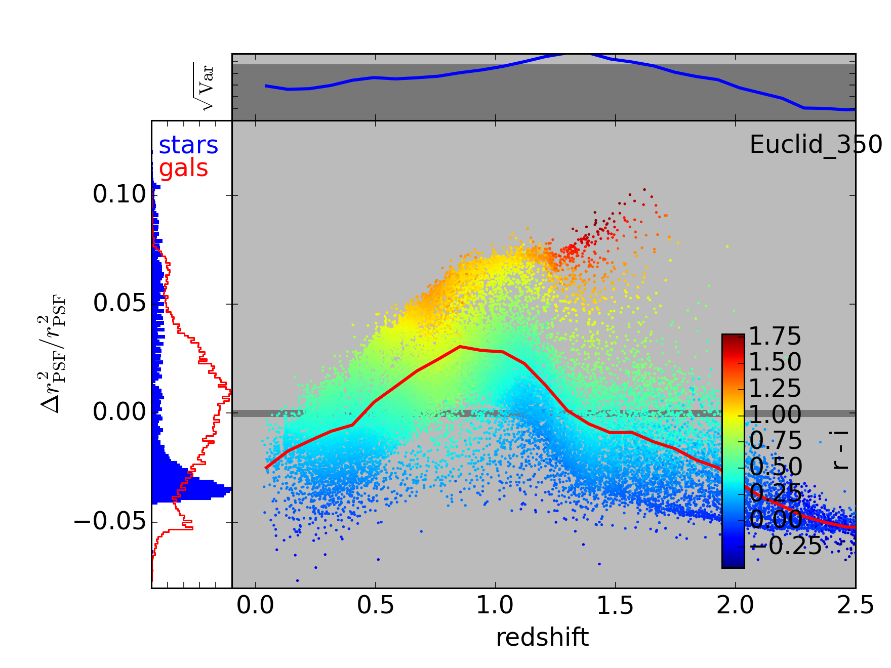
The last plot here, for the Euclid telescope, is slightly misleading since we generated a catalog appropriate for LSST, and Euclid will be a much shallower survey. However, the peak of the Euclid chromatic PSF bias is around redshift 1.0, where Euclid will still be quite sensitive. Also notice that the symbol colors for this plot represent LSST $r$ - $i$ color. The proposed Euclid footprint will overlap the LSST footprint by about 5000 square degrees.

Notice also that while chromatic biases are clearly correlated with $r$ - $i$ , they aren’t perfectly correlated. That is, for a given chromatic bias, or horizontal cut across the above scatter plots, more than one $r$ - $i$ color, or symbol color, occurs.

Back