Model Fitting Bias
The previous pages’ results looked purely at analytic expectations for chromatic biases, based on propagating expected shifts in PSF second moments into ellipticity defined as an unweighted combination of deconvolved surface brightness profile second moments. This approach assumes that PSF deconvolution will succeed exactly, something difficult to achieve in practice. On this page, we investigate a second way to estimate the impact of chromatic PSF biases, based on simulated images of galaxies affected by chromatic PSFs.
Ring test
The alternative way to estimate shear bias induced by chromatic effects is to simulate sheared galaxy images using the true (galactic) SED, and then attempt to recover the simulated galactic ellipticities while pretending that the galaxy instead had a stellar SED. A ring test (Nakajima & Bernstein 2007) is a specific prescription for such a suite of simulations designed to rapidly converge to the correct (though biased) shear calibration parameters. The test gets its name from the arrangement of galaxy shapes used in the simulated images, which form a ring in ellipticity space centered at the origin (i.e. |e| is constant), before any shear is applied. By choosing intrinsic ellipticities that exactly average to zero, the results of the test converge faster than for randomly (though isotropically) chosen ellipticities that only average to zero statistically.
The general procedure can be implemented as follows:
- Choose an input “true” reduced shear \(g\).
- Choose a pre-sheared galaxy ellipticity \(e^\mathrm{int}\) on the ring.
- Compute the sheared galaxy ellipticity \( e^\mathrm{obs} = \frac{e^\mathrm{int} + g}{1+g^*e^\mathrm{int}} \)
- Generate the target image using the chromatic PSF, assuming the SED is galactic.
- Fit a model to this target image pretending the SED is instead stellar. (Do this by varying the model parameters that define the galaxy, including, e.g., \(e^\mathrm{obs}\))
- Repeat steps 3-5 using the opposite pre-sheared ellipticity: \( e^\mathrm{int} \rightarrow -e^\mathrm{int} \).
- Repeat steps 2-6 for as many values around the ellipticity ring as desired. Typically these values are uniformly spaced.
- Average together all recorded output ellipticity \(e^\mathrm{obs}\) values. This is the (biased by chromaticity) estimate for the shear \(\hat{g}\).
- Repeat steps 1-8 to map out the relation \(g \rightarrow \hat{g} \). \(1+m\) and \(c\) are then the slope and intercept of this relation.
Implementation in Chroma
In Chroma, the bin/simulations/one_ring_test.py script carries out exactly the above procedure.
Let’s run this script with the default options (i.e. no command line options).
$ cd CHROMA_DIR/bin/simulations/
$ python one_ring_test.py

General settings
----------------
stamp size: 31
pixel scale: 0.2 arcsec/pixel
ring test angles: 3

Spectra settings
----------------
Data directory: ../../data/
Filter: filters/LSST_r.dat
Filter effective wavelength: 619.914042861
Thinning with relative error: 1e-08
Galaxy SED: SEDs/KIN_Sa_ext.ascii
Galaxy redshift: 0.0
Star SED: SEDs/ukg5v.ascii

Spectra chromatic biases
------------------------
Vstar: 0.006430 arcsec^2
Vgal: 0.006246 arcsec^2
r^2_{PSF,gal}/r^2_{PSF,*}: 0.997788

Gaussian PSF settings
---------------------
PSF phi: 0.0 degrees
PSF ellip: 0.0
PSF FWHM: 0.7 arcsec
PSF sqrt(r^2): 0.420392843075
PSF alpha: -0.2

Observation settings
--------------------
zenith angle: 45.0 degrees
parallactic angle: 0.0 degrees

Galaxy settings
---------------
Galaxy Sersic index: 0.5
Galaxy ellipticity: 0.3
Galaxy sqrt(r^2): 0.27 arcsec
Galaxy HLR:  0.225 arcsec
Galaxy PSF-convolved FWHM:  0.869 +/-  0.001 arcsec

Shear Calibration Results
-------------------------
                m1        m2        c1        c2
analytic    0.0079    0.0079    0.0013    0.0000
ring        0.0083    0.0083    0.0014   -0.0000

Survey requirements
DES         0.0080    0.0080    0.0025    0.0025
LSST        0.0030    0.0030    0.0015    0.0015
The script first reports information about what simulation it’s going to run; things like the size of the pixels, the zenith angle used for DCR, and morphological and spectral properties of the simulated galaxy and PSF. Most of these properties are configurable. The lines labeled “analytic” and “ring” are the actual output of the program. The “analytic” line shows the estimates for the shear calibration parameters from analytic formulae, and the “ring” line shows the values obtained from the ring test. In this case there’s a slight disagreement between these, though clearly both estimates are in the same ballpark. The last two lines show the nominal maximum values of and tolerable for the DES and LSST surveys. Note that these are the final tolerances, including many systematic effects beyond chromatic PSF biases. We should therefore strive to correct chromatic effects to well below this threshold.
Let’s look at what options are configurable for this test:
usage: one_ring_test.py [-h] [--datadir DATADIR] [-s STARSPEC] [-g GALSPEC]
                        [-f FILTER] [-z REDSHIFT] [--thin THIN]
                        [-za ZENITH_ANGLE] [-q PARALLACTIC_ANGLE]
                        [--kolmogorov | --moffat] [--PSF_beta PSF_BETA]
                        [--PSF_FWHM PSF_FWHM | --PSF_r2 PSF_R2]
                        [--PSF_phi PSF_PHI] [--PSF_ellip PSF_ELLIP]
                        [-n SERSIC_N] [--gal_ellip GAL_ELLIP]
                        [--gal_r2 GAL_R2 | --gal_convFWHM GAL_CONVFWHM | --gal_HLR GAL_HLR]
                        [--nring NRING] [--pixel_scale PIXEL_SCALE]
                        [--stamp_size STAMP_SIZE] [--image_x0 IMAGE_X0]
                        [--image_y0 IMAGE_Y0] [--slow] [--alpha ALPHA]
                        [--noDCR] [--diagnostic DIAGNOSTIC] [--hsm]
                        [--perturb] [--quiet]
                        [--maximum_fft_size MAXIMUM_FFT_SIZE]

optional arguments:
  -h, --help            show this help message and exit
  --datadir DATADIR     directory to find SED and filter files.
  -s STARSPEC, --starspec STARSPEC
                        stellar spectrum to use when fitting (Default
                        'SEDs/ukg5v.ascii'x)
  -g GALSPEC, --galspec GALSPEC
                        galactic spectrum used to create target image (Default
                        'SEDs/KIN_Sa_ext.ascii')
  -f FILTER, --filter FILTER
                        filter for simulation (Default 'filters/LSST_r.dat')
  -z REDSHIFT, --redshift REDSHIFT
                        galaxy redshift (Default 0.0)
  --thin THIN           Thin but retain bandpass integral accuracy to this
                        relative amount. (Default: 1.e-8).
  -za ZENITH_ANGLE, --zenith_angle ZENITH_ANGLE
                        zenith angle in degrees for differential chromatic
                        refraction computation (Default: 45.0)
  -q PARALLACTIC_ANGLE, --parallactic_angle PARALLACTIC_ANGLE
                        parallactic angle in degrees for differential
                        chromatic refraction computation (Default: 0.0)
  --kolmogorov          Use Kolmogorov PSF (Default Gaussian)
  --moffat              Use Moffat PSF (Default Gaussian)
  --PSF_beta PSF_BETA   Set beta parameter of Moffat profile PSF. (Default
                        2.5)
  --PSF_FWHM PSF_FWHM   Set FWHM of PSF in arcsec (Default 0.7).
  --PSF_r2 PSF_R2       Override PSF_FWHM with second moment radius sqrt(r^2).
  --PSF_phi PSF_PHI     Set position angle of PSF in degrees (Default 0.0).
  --PSF_ellip PSF_ELLIP
                        Set ellipticity of PSF (Default 0.0)
  -n SERSIC_N, --sersic_n SERSIC_N
                        Sersic index (Default 0.5)
  --gal_ellip GAL_ELLIP
                        Set ellipticity of galaxy (Default 0.3)
  --gal_r2 GAL_R2       Set galaxy second moment radius sqrt(r^2) in arcsec
                        (Default 0.27)
  --gal_convFWHM GAL_CONVFWHM
                        Override gal_r2 by setting galaxy PSF-convolved FWHM.
  --gal_HLR GAL_HLR     Override gal_r2 by setting galaxy half-light-radius.
  --nring NRING         Set number of angles in ring test (Default 3)
  --pixel_scale PIXEL_SCALE
                        Set pixel scale in arcseconds (Default 0.2)
  --stamp_size STAMP_SIZE
                        Set postage stamp size in pixels (Default 31)
  --image_x0 IMAGE_X0   Image origin x-offset in pixels (Default 0.0)
  --image_y0 IMAGE_Y0   Image origin y-offset in pixels (Default 0.0)
  --slow                Use ChromaticSersicTool (somewhat more careful)
                        instead of FastChromaticSersicTool.
  --alpha ALPHA         Power-law index for chromatic seeing (Default: -0.2)
  --noDCR               Exclude differential chromatic refraction (DCR) in
                        PSF. (Default: include DCR)
  --diagnostic DIAGNOSTIC
                        Filename to which to write diagnostic images (Default:
                        '')
  --hsm                 Use HSM regaussianization to estimate ellipticity
  --perturb             Use PerturbFastChromaticSersicTool to estimate
                        ellipticity
  --quiet               Don't print settings
  --maximum_fft_size MAXIMUM_FFT_SIZE
                        Maximum FFT GalSim is willing to do.
There are lots of possible variations to investigate! Here’s a particularly interesting one:
$ python one_ring_test.py -n 4.0
...

Shear Calibration Results
-------------------------
                m1        m2        c1        c2
analytic    0.0079    0.0079    0.0013    0.0000
ring        0.0171    0.0166    0.0051    0.0000

Survey requirements
DES         0.0080    0.0080    0.0025    0.0025
LSST        0.0030    0.0030    0.0015    0.0015
That’s interesting. Changing the Sersic index of the simulated galaxy had no affect on the analytic
results. That makes sense since the analytic formulae only care about the galaxy’s second moment
radius \(r^2\mathrm{gal} = Ixx + Iyy \), not on the details of its surface brightness profile.
The one_ring_test.py script is specifically designed to keep \( r^2\mathrm{gal} \) fixed as the
Sersic index is varied (though this can be changed using the --gal_HLR or --gal_convFWHM keyword
arguments). The results for the ring test changed by quite a bit, however. What’s going on? We
can investigate using the command line option --diagnostic and the script
plot_ring_diagnostic.py:
$ python one_ring_test.py -n 0.5 --diagnostic n0.5.fits
$ python one_ring_test.py -n 4.0 --diagnostic n4.0.fits --maximum_fft_size 16384
$ python plot_ring_diagnostic.py --help
usage: plot_ring_diagnostic.py [-h] infile [outprefix]

positional arguments:
  infile      Input diagnostic fits filename.
  outprefix   Output PNG filename prefix. (Default: output/ring_diagnostic)

optional arguments:
  -h, --help  show this help message and exit
$ python plot_ring_diagnostic.py n4.0.fits n4.0
$ python plot_ring_diagnostic.py n0.5.fits n0.5
$ ls *.png
n0.5-g1-0.0-g2-0.0-beta0.0.png              n4.0-g1-0.0-g2-0.0-beta0.0.png
n0.5-g1-0.0-g2-0.0-beta1.0471975512.png     n4.0-g1-0.0-g2-0.0-beta1.0471975512.png
n0.5-g1-0.0-g2-0.0-beta2.09439510239.png    n4.0-g1-0.0-g2-0.0-beta2.09439510239.png
n0.5-g1-0.0-g2-0.0-beta3.14159265359.png    n4.0-g1-0.0-g2-0.0-beta3.14159265359.png
n0.5-g1-0.0-g2-0.0-beta4.18879020479.png    n4.0-g1-0.0-g2-0.0-beta4.18879020479.png
n0.5-g1-0.0-g2-0.0-beta5.23598775598.png    n4.0-g1-0.0-g2-0.0-beta5.23598775598.png
n0.5-g1-0.01-g2-0.02-beta0.0.png            n4.0-g1-0.01-g2-0.02-beta0.0.png
n0.5-g1-0.01-g2-0.02-beta1.0471975512.png   n4.0-g1-0.01-g2-0.02-beta1.0471975512.png
n0.5-g1-0.01-g2-0.02-beta2.09439510239.png  n4.0-g1-0.01-g2-0.02-beta2.09439510239.png
n0.5-g1-0.01-g2-0.02-beta3.14159265359.png  n4.0-g1-0.01-g2-0.02-beta3.14159265359.png
n0.5-g1-0.01-g2-0.02-beta4.18879020479.png  n4.0-g1-0.01-g2-0.02-beta4.18879020479.png
n0.5-g1-0.01-g2-0.02-beta5.23598775598.png  n4.0-g1-0.01-g2-0.02-beta5.23598775598.png
We’ve created a bunch of diagnostic plots for each step of the two ring tests we’ve run. Let’s look
at n0.5-g1-0.0-g2-0.0-beta1.0471975512.png, which corresponds to steps 4 and 5 of the ring test
procedure where \(g = 0.0\), \(n = 0.5 \)(i.e. the galaxy is Gaussian), and
\(\beta = 1.0471975512\) (i.e. the galaxy is oriented with its major axis at an angle of
to the x axis).
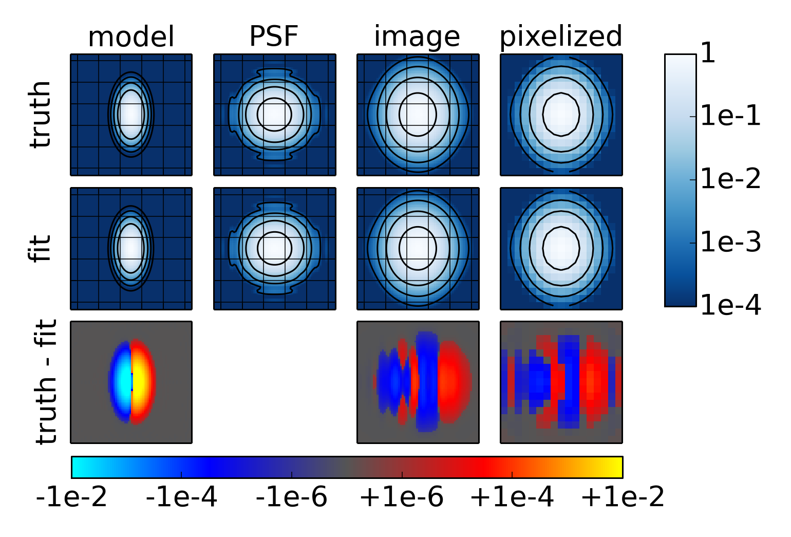
Let’s take this figure one panel at a time. The first panel at the top left is the target galaxy model, post-shear but pre-PSF-convolution. To the right is the effective PSF when the SED is galactic. To the right of that is the convolved image, and finally the rightmost panel is the pixelized and convolved image. The second row shows the same images but for the fitting step of the ring test procedure (step 5). That is, the effective PSF is for the stellar SED instead of the galactic SED, and the model is the result of the fitting procedure; the images are the convolved and pixelized versions of these. Not much difference, huh? That’s just an indication that the chromatic biases we’re studying are tiny, and by extension that the requirements for LSST are incredibly strict.
The final row shows the residuals between the target image generated assuming a galactic SED, and the best fit when pretending that the SED is stellar. Note that the scale bar for this row is different than the top rows and somewhat unusual in that it’s displaying both positive and negative values logarithmically (with a linear transition region in the middle).
The residuals in the image columns say something about how well we were able to deconvolve the stellar SED effective PSF from the target image. If the deconvolution proceeded perfectly, then the images columns in both the “truth” and “fit” rows would be exactly equal to each other, and there wouldn’t be any residuals in the images columns. The fact that the residuals there are not zero says that the deconvolution is only approximate.
Another way to think about this is that the deconvolution by the stellar PSF of the Sersic profile convolved by the galactic PSF, is no long exactly describable as a Sersic profile; it’s something more complicated. Since we’re restricting the best fit model to be a Sersic profile, we therefore make some small amount of error in this deconvolution.
Let’s see what the \(n=4.0\) case looks like:
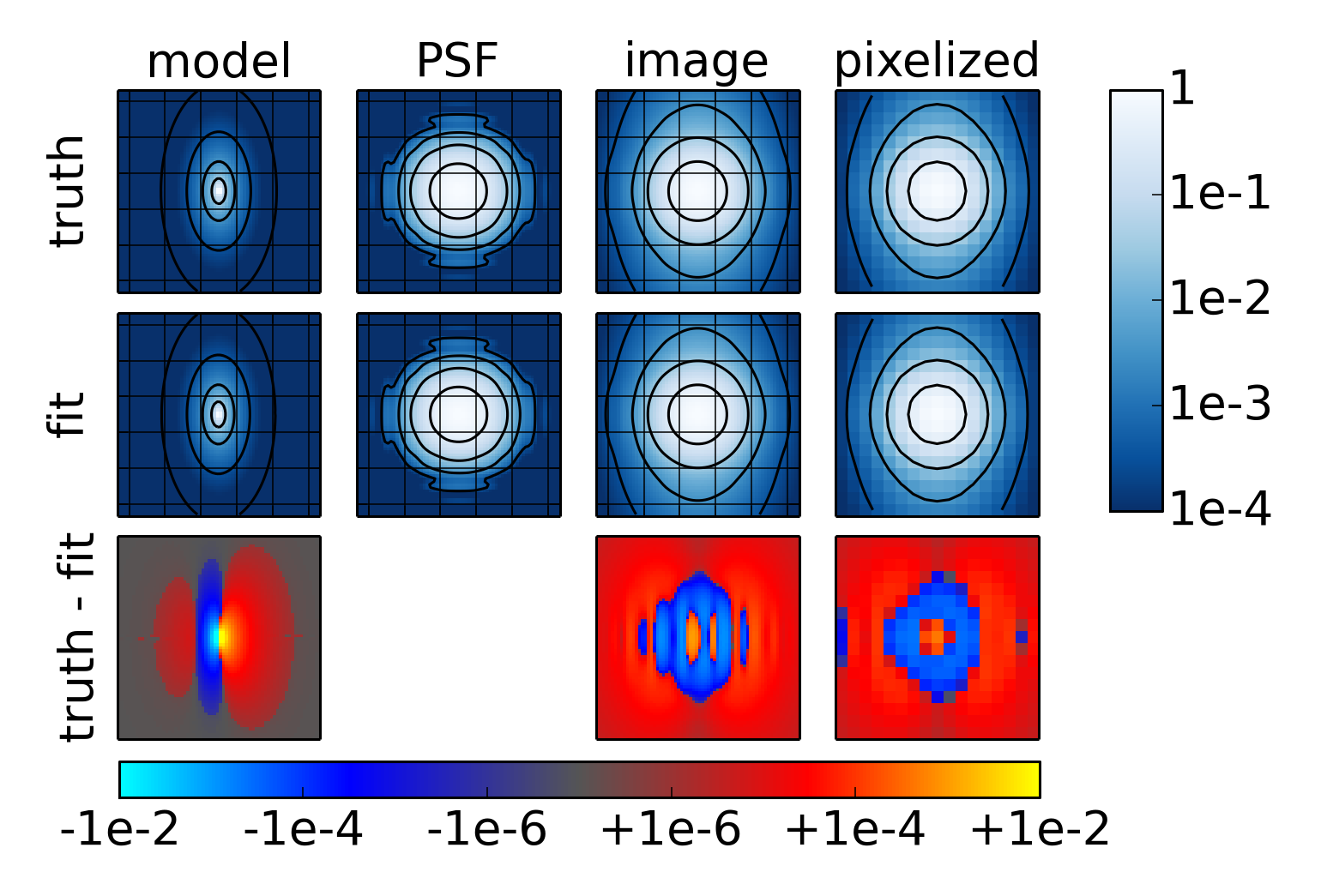
The residuals are clearly larger in this case. That is, the bias due to our choice of model is larger when \(n = 4.0\) than when \(n = 0.5\). This explains why the ring test results are further from the analytic results for \(n = 4.0\).