Table of Contents

• 1  Generate random data and add to catalog

• 2  Match catalogs

• 3  Find the scaling relation between the masses of the two catalogs

• 4  Recovery rate

  • 4.1  Panels plots

• 5  Difference with threshold mass

• 6  Difference catalog mass

Intrinsic Completeness

When two catalogs with different mass proxies and a threshold mass proxy, there is a intrinsic completeness limitaion on the relative completeness of the catalogs.

We can associate the mass proxy relation of two catalog with:

\[P(M_2|M_1)\frac{dn}{dM_1}=P(M_1|M_2)\frac{dn}{dM_2},\]

where \(P(M_1|M_2)\) is the probability of having a catalog 1 cluster with mass \(M_1\) given a catalog 2 cluster with mass \(M_2\), and \(\frac{dn}{dM_1}\) is the mass function of catalog 1. Then the number of catalog 1 cluster with mass \(M_1\) can be computed as:

\[n(M_1)=\int_{-\infty}^{\infty}dM_2 \frac{dn}{dM_2}P(M_1|M_2).\]

However, if catalog 2 has a cut given by some threshold \(M_2^{th}\), the number of clusters we can expect to measure is:

\[n_{M_2^{th}}(M_1)=\int_{M_2^{th}}^{\infty}dM_2 \frac{dn}{dM_2}P(M_1|M_2),\]

and the relative completeness resulting is:

\[c_{M_2^{th}}(M_1)= \frac{n_{M_2^{th}}(M_1)}{n(M_1)}= \frac {\int_{M_2^{th}}^{\infty}dM_2 \frac{dn}{dM_2}P(M_1|M_2)} {\int_{-\infty}^{\infty}dM_2 \frac{dn}{dM_2}P(M_1|M_2)}.\]

We can see that this is just the integral of \(P(M_1|M_2)\) weighted by the mass function \(\frac{dn}{dM_2}\). In an approximation where this factor presents minor effect (see the appendix), we can estimate this completeness as:

\[c_{M_2^{th}}(M_1)= \frac {\int_{M_2^{th}}^{\infty}dM_2 P(M_1|M_2)} {\int_{-\infty}^{\infty}dM_2 P(M_1|M_2)}.\]

This is the estimation that can be done in clevar.

%load_ext autoreload
%autoreload 2

import numpy as np
import pylab as plt
from IPython.display import Markdown as md

Generate random data and add to catalog

# For reproducibility
np.random.seed(1)

from support import gen_cluster
logm_scatter = 0.1
input1, input2 = gen_cluster(lnm_scatter=logm_scatter*np.log(10))

Initial number of clusters (logM>12.70): 1,925
Clusters in catalog1: 908
Clusters in catalog2: 945

from clevar import ClCatalog
c1 = ClCatalog('Cat1', ra=input1['RA'], dec=input1['DEC'], z=input1['Z'], mass=input1['MASS'],
            mass_err=input1['MASS_ERR'], z_err=input1['Z_ERR'])
c2 = ClCatalog('Cat2', ra=input2['RA'], dec=input2['DEC'], z=input2['Z'], mass=input2['MASS'],
            mass_err=input2['MASS_ERR'], z_err=input2['Z_ERR'])
# Format for nice display
for c in ('ra', 'dec', 'z', 'z_err'):
    c1[c].info.format = '.2f'
    c2[c].info.format = '.2f'
for c in ('mass', 'mass_err'):
    c1[c].info.format = '.2e'
    c2[c].info.format = '.2e'

/home/aguena/.local/lib/python3.9/site-packages/clevar-0.13.2-py3.9.egg/clevar/catalog.py:267: UserWarning: id column missing, additional one is being created.
  warnings.warn(

Match catalogs

from clevar.match import ProximityMatch
from clevar.cosmology import AstroPyCosmology

match_config = {
    'type': 'cross', # options are cross, cat1, cat2
    'which_radius': 'max', # Case of radius to be used, can be: cat1, cat2, min, max
    'preference': 'angular_proximity', # options are more_massive, angular_proximity or redshift_proximity
    'catalog1': {'delta_z':.2,
                'match_radius': '10 arcsec'
                },
    'catalog2': {'delta_z':.2,
                'match_radius': '10 arcsec'
                }
}

mt = ProximityMatch()
mt.match_from_config(c1, c2, match_config)

## ClCatalog 1
## Prep mt_cols
* zmin|zmax from config value
* ang radius from set scale

## ClCatalog 2
## Prep mt_cols
* zmin|zmax from config value
* ang radius from set scale

## Multiple match (catalog 1)
Finding candidates (Cat1)
* 822/908 objects matched.

## Multiple match (catalog 2)
Finding candidates (Cat2)
* 822/945 objects matched.

## Finding unique matches of catalog 1
Unique Matches (Cat1)
* 822/908 objects matched.

## Finding unique matches of catalog 2
Unique Matches (Cat2)
* 822/945 objects matched.
Cross Matches (Cat1)
* 822/908 objects matched.
Cross Matches (Cat2)
* 822/945 objects matched.

Find the scaling relation between the masses of the two catalogs

from clevar.match_metrics import scaling

zbins = np.linspace(0, 2, 21)
mbins = np.logspace(13, 14, 5)

info2_mr = scaling.mass_density_metrics(
    c2, c1, 'cross', ax_rotation=45,
    add_err=False, plt_kwargs={'s':5},
    mask1=c2['mass']>2e13,
    add_fit=True, fit_bins1=20, fit_bins2=10, fit_err2=None,
    bins1=20)

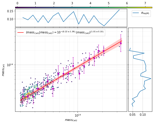
The output of scaling.mass* functions contains a ['fit']['func_dist_interp'] element representing \(P(M_1|M_2)\), which can be passed directly to the recovery rates to estimate the intrinsic completeness.

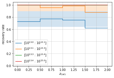
Recovery rate

Compute recovery rates, they are computed in mass and redshift bins. To add the intrinsic completeness, also pass the following arguments: * p_m1_m2: \(P(M_1|M_2)\) - Probability of having a catalog 1 cluster with mass \(M_1\) given a catalog 2 cluster with mass \(M_2\). * min_mass2: Minimum mass (proxy) of the other catalog.

from clevar.match_metrics import recovery

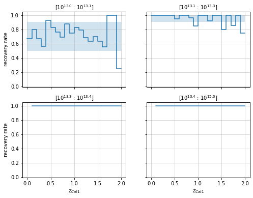
When plotted as a function of redshift with mass bins, it will add shaded reagions corresponding to the completeness of each mass bin:

zbins = np.linspace(0, 2, 5)
mbins = np.append(np.logspace(13, 13.4, 4), 1e15)
info = recovery.plot(c1, 'cross', zbins, mbins,
                     p_m1_m2=info2_mr['fit']['func_dist_interp'], min_mass2=1e13)
plt.show()

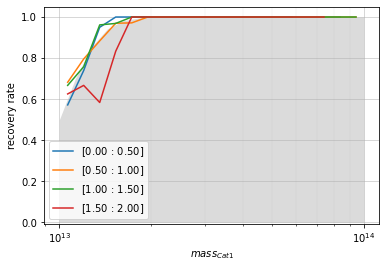
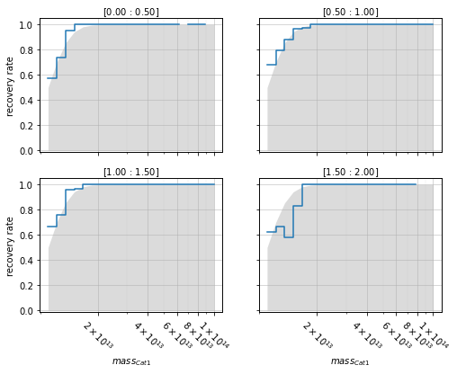
When plotted as a function of mass with redshift bins, it will add a shaded region correspong to the intrinsic completeness as a function of mass:

zbins = np.linspace(0, 2, 5)
mbins = np.logspace(13, 14, 20)
info = recovery.plot(
    c1, 'cross', zbins, mbins,
    shape='line', transpose=True,
    p_m1_m2=info2_mr['fit']['func_dist_interp'], min_mass2=1e13)

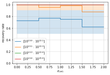
In this case specifically, we do know the true distribution \(P(M_2|M_1)\) that was used by gen_cluster to generate the clusters. So we can compare these estimated results with the “true” intrinsic completeness:

p_m1_m2 = lambda m1, m2: np.exp(-0.5*(np.log10(m2/m1))**2/logm_scatter**2)/np.sqrt(2*np.pi*logm_scatter**2)

# By redshift
zbins = np.linspace(0, 2, 5)
mbins = np.append(np.logspace(13, 13.4, 4), 1e15)
info = recovery.plot(c1, 'cross', zbins, mbins,
                     p_m1_m2=p_m1_m2, min_mass2=1e13)
plt.show()

# By mass
zbins = np.linspace(0, 2, 5)
mbins = np.logspace(13, 14, 20)
info = recovery.plot(
    c1, 'cross', zbins, mbins,
    shape='line', transpose=True,
    p_m1_m2=p_m1_m2, min_mass2=1e13)

# By redshift
zbins = np.linspace(0, 2, 5)
mbins = np.append(np.logspace(13, 13.4, 4), 1e15)
info = recovery.plot(c1, 'cross', zbins, mbins,
                     p_m1_m2=p_m1_m2, min_mass2=1e13)
plt.show()

# By mass
zbins = np.linspace(0, 2, 5)
mbins = np.logspace(13, 14, 20)
info = recovery.plot(
    c1, 'cross', zbins, mbins,
    shape='line', transpose=True,
    p_m1_m2=p_m1_m2, min_mass2=1e13)

Panels plots

You can also have a panel for each bin:

zbins = np.linspace(0, 2, 21)
mbins = np.append(np.logspace(13, 13.4, 4), 1e15)
info = recovery.plot_panel(c1, 'cross', zbins, mbins,
                           p_m1_m2=p_m1_m2, min_mass2=1e13)

zbins = np.linspace(0, 2, 5)
mbins = np.logspace(13, 14, 20)
info = recovery.plot_panel(c1, 'cross', zbins, mbins, transpose=True,
                          p_m1_m2=p_m1_m2, min_mass2=1e13)

Appendix: Estimating deviation in completeness approximation

Here we can compute the deviation of disregarding the mass function factor in the intrinsic completeness estimation, i. e. comparing:

\[c(M)= \frac {\int_{M_2^{th}}^{\infty}dM_2 \frac{dn}{dM_2}P(M_1|M_2)} {\int_{-\infty}^{\infty}dM_2 \frac{dn}{dM_2}P(M_1|M_2)},\]

with

\[c_{approx}(M_1)= \frac {\int_{M_2^{th}}^{\infty}dM_2 P(M_1|M_2)} {\int_{-\infty}^{\infty}dM_2 P(M_1|M_2)}.\]

# Mass function approximation, derived from DC2 simulation:
dn_dlogm = lambda x: 10**np.poly1d([ -0.4102,   9.6586, -52.4729])(x)

# Gaussian distribution for logm
p_m1_m2 = lambda m1, m2: np.exp(-0.5*(np.log10(m2/m1))**2/logm_scatter**2)/np.sqrt(2*np.pi*logm_scatter**2)

from scipy.integrate import quad_vec

# Limits for integrals
min_log_mass2_norm = 10
max_log_mass2 = 16

# Normalized integral
def normalized_integral(m1, m2_th, func):
    integ = quad_vec(func, np.log10(m2_th), max_log_mass2, epsabs=1e-50)[0]
    norm = quad_vec(func, min_log_mass2_norm, max_log_mass2, epsabs=1e-50)[0]
    if hasattr(integ, '__len__'):
        integ[norm>0] /= norm[norm>0]
    else:
        integ = integ/norm if norm>0 else integ
    return integ

# Intrinsic completenss
comp_full = lambda m1, m2_th: normalized_integral(
    m1, m2_th, lambda logm2: p_m1_m2(m1, 10**logm2)*dn_dlogm(logm2))

# Intrinsic completeness disregarding mass function
comp_approx = lambda m1, m2_th: normalized_integral(
    m1, m2_th, lambda logm2: p_m1_m2(m1, 10**logm2))

We can estimate the difference as a function of \(M_1\) or \(M_2^{th}\). We will see both below.

Difference with threshold mass

Here we want to see the difference of this approximations as a function of \(M_2^{th}\).

m1 = 1e13

md(f'We start by fixing $M_1$ at $10^{{{np.log10(m1):.1f}}}$'
  r' and evaluating the difference of the arguments $\frac{dn}{dM_2}P(M_1|M_2)$ vs $P(M_1|M_2)$:')

We start by fixing \(M_1\) at \(10^{13.0}\) and evaluating the difference of the arguments \(\frac{dn}{dM_2}P(M_1|M_2)\) vs \(P(M_1|M_2)\):

m2_vec = np.logspace(12, 15, 500)
norm1 = quad_vec(lambda logm2: p_m1_m2(m1, 10**logm2)*dn_dlogm(logm2),
    min_log_mass2_norm, max_log_mass2, epsabs=1e-50)[0]
norm2 = quad_vec(lambda logm2: p_m1_m2(m1, 10**logm2),
    min_log_mass2_norm, max_log_mass2, epsabs=1e-50)[0]

plt.plot(m2_vec, p_m1_m2(m1, m2_vec)*dn_dlogm(np.log10(m2_vec))/norm1,
         label=r'$\frac{dn}{dM_2}P(M_1|M_2)$')
plt.plot(m2_vec, p_m1_m2(m1, m2_vec)/norm2, label='$P(M_1|M_2)$')


plt.axvline(m1, ls='--', color='r')
plt.text(m1, 0, '$M_1$', color='r')

plt.xscale('log')
plt.xlabel('$M_2$')
plt.ylabel('kernel')
plt.legend(fontsize=16)
plt.show()

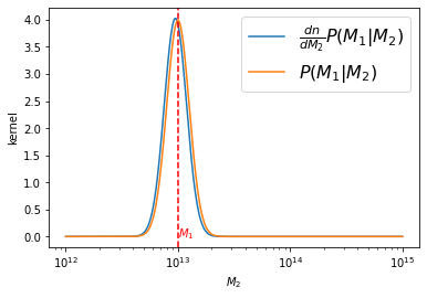
There is only a small shift in the argument to be integrated.

When making the integrals:

m2_th_vec = np.logspace(12, 14, 100)

int_full_m1fix = np.array([comp_full(m1, m2) for m2 in m2_th_vec])
int_approx_m1fix = np.array([comp_approx(m1, m2) for m2 in m2_th_vec])

and checking the difference:

f, axes = plt.subplots(2, figsize=(6, 8), sharex=True)

axes[0].plot(m2_th_vec, int_full_m1fix, label=r'$\frac{dn}{dM_2}P(M_2|M_1)$')
axes[0].plot(m2_th_vec, int_approx_m1fix, label='$P(M_2|M_1)$')

diff_m1fix = int_approx_m1fix-int_full_m1fix
axes[1].plot(m2_th_vec, diff_m1fix)

axes[0].legend(fontsize=16)
axes[0].set_ylabel('$c_{M_2^{th}}(M_1=10^{13})$')
axes[1].set_ylabel('$difference$')
axes[1].set_xlabel('$M_2^{th}$')


for ax in axes:
    ax.set_xscale('log')
    ax.axvline(m1, ls='--', color='r')
    ax.text(m1, 0, '$M_1$', color='r')

plt.show()

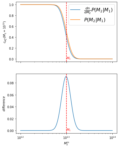
md(f'the maximum difference is of {diff_m1fix.max():.4f}. '
   f'Therefore the approximation only deviates by {diff_m1fix.max()*100:.0f}%,'
   ' and it occurs at $M_2^{th}$=$M_1$')

the maximum difference is of 0.0910. Therefore the approximation only deviates by 9%, and it occurs at \(M_2^{th}\)=\(M_1\)

Difference catalog mass

Here we want to see the difference of this approximations as a function of \(M_1\).

m2_th = 1e13

md(f'We start by setting $M_2^{{th}}$ at $10^{{{np.log10(m2_th):.1f}}}$'
  r' and evaluating the difference of the arguments $\frac{dn}{dM_2}P(M_1|M_2)$ vs $P(M_1|M_2)$:')

We start by setting \(M_2^{th}\) at \(10^{13.0}\) and evaluating the difference of the arguments \(\frac{dn}{dM_2}P(M_1|M_2)\) vs \(P(M_1|M_2)\):

m1_vec = np.logspace(12, 14, 201)

int_full_m2fix = comp_full(m1_vec, m2_th)
int_approx_m2fix = comp_approx(m1_vec, m2_th)

f, axes = plt.subplots(2, figsize=(6, 8), sharex=True)

axes[0].plot(m1_vec, int_full_m2fix, label=r'$\frac{dn}{dM_2}P(M_1|M_2)$')
axes[0].plot(m1_vec, int_approx_m2fix, label='$P(M_1|M_2)$')

diff_m2fix = int_approx_m2fix-int_full_m2fix
axes[1].plot(m1_vec, diff_m2fix)

axes[0].legend(fontsize=16)
axes[0].set_ylabel('$c_{M_2^{th}=10^{13}}(M_1)$')
axes[1].set_ylabel('$difference$')
axes[1].set_xlabel('$M_1$')
for ax in axes:
    ax.set_xscale('log')
    ax.axvline(m2_th, ls='--', color='r')
    ax.text(m2_th, 0, '$M_2^{th}$', color='r')

plt.show()

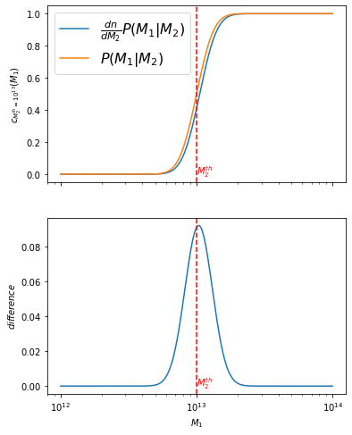
md(f'The maximum difference is of {diff_m2fix.max():.4f}. '
   f'Therefore the approximation only deviates by {diff_m2fix.max()*100:.0f}%,'
   ' and it occurs at $M_1$=$M_2^{th}$')

The maximum difference is of 0.0918. Therefore the approximation only deviates by 9%, and it occurs at \(M_1\)=\(M_2^{th}\)