Metrics of matching (simple)
Example of the functions to plot match_metrics of matching.
%load_ext autoreload
%autoreload 2
import numpy as np
import pylab as plt
Generate random data and add to catalog
# For reproducibility
np.random.seed(1)
from support import gen_cluster
input1, input2 = gen_cluster(ra_min=0, ra_max=30, dec_min=0, dec_max=30)
Initial number of clusters (logM>12.48): 2,740
Clusters in catalog1: 835
Clusters in catalog2: 928
from clevar import ClCatalog
c1 = ClCatalog('Cat1', ra=input1['RA'], dec=input1['DEC'], z=input1['Z'], mass=input1['MASS'],
            mass_err=input1['MASS_ERR'], z_err=input1['Z_ERR'])
c2 = ClCatalog('Cat2', ra=input2['RA'], dec=input2['DEC'], z=input2['Z'], mass=input2['MASS'],
            mass_err=input2['MASS_ERR'], z_err=input2['Z_ERR'])
# Format for nice display
for c in ('ra', 'dec', 'z', 'z_err'):
    c1[c].info.format = '.2f'
    c2[c].info.format = '.2f'
for c in ('mass', 'mass_err'):
    c1[c].info.format = '.2e'
    c2[c].info.format = '.2e'
/home/aguena/.local/lib/python3.9/site-packages/clevar-0.13.2-py3.9.egg/clevar/catalog.py:267: UserWarning: id column missing, additional one is being created.
  warnings.warn(
Match catalogs
from clevar.match import ProximityMatch
from clevar.cosmology import AstroPyCosmology

match_config = {
    'type': 'cross', # options are cross, cat1, cat2
    'which_radius': 'max', # Case of radius to be used, can be: cat1, cat2, min, max
    'preference': 'angular_proximity', # options are more_massive, angular_proximity or redshift_proximity
    'catalog1': {'delta_z':.2,
                'match_radius': '1 mpc'
                },
    'catalog2': {'delta_z':.2,
                'match_radius': '10 arcsec'
                }
}

cosmo = AstroPyCosmology()
mt = ProximityMatch()
mt.match_from_config(c1, c2, match_config, cosmo=cosmo)
## ClCatalog 1
## Prep mt_cols
* zmin|zmax from config value
* ang radius from set scale

## ClCatalog 2
## Prep mt_cols
* zmin|zmax from config value
* ang radius from set scale

## Multiple match (catalog 1)
Finding candidates (Cat1)
* 719/835 objects matched.

## Multiple match (catalog 2)
Finding candidates (Cat2)
* 721/928 objects matched.

## Finding unique matches of catalog 1
Unique Matches (Cat1)
* 719/835 objects matched.

## Finding unique matches of catalog 2
Unique Matches (Cat2)
* 720/928 objects matched.
Cross Matches (Cat1)
* 719/835 objects matched.
Cross Matches (Cat2)
* 719/928 objects matched.
Recovery rate
Compute recovery rates, they are computed in mass and redshift bins. There are several ways they can be displayed: - Single panel with multiple lines - Multiple panels - 2D color map
from clevar.match_metrics import recovery
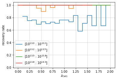
Simple plot
The recovery rates are shown as a function of redshift in mass bins. They can be displayed as a continuous line or with steps:
zbins = np.linspace(0, 2, 21)
mbins = np.logspace(13, 14, 5)
info = recovery.plot(c1, 'cross', zbins, mbins, shape='steps')
plt.show()
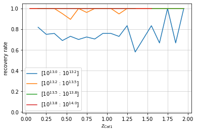
info = recovery.plot(c1, 'cross', zbins, mbins, shape='line')
plt.show()
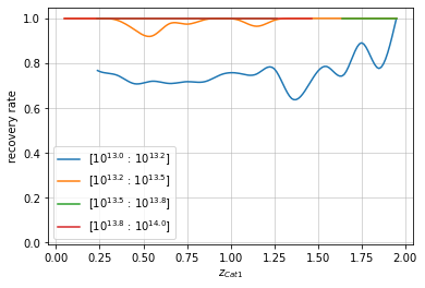
You can also smoothen the lines of the plot:
info = recovery.plot(c1, 'cross', zbins, mbins, shape='line',
                     plt_kwargs={'n_increase':3})
plt.show()
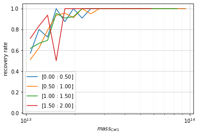
They can also be transposed to be shown as a function of mass in redshift bins.
zbins = np.linspace(0, 2, 5)
mbins = np.logspace(13, 14, 20)
info = recovery.plot(c1, 'cross', zbins, mbins,
                     shape='line', transpose=True)
The full information of the recovery rate histogram in a dictionay containing:
data: Binned data used in the plot. It has the sections:recovery: Recovery rate binned with (bin1, bin2). bins where no cluster was found have nan value.edges1: The bin edges along the first dimension.edges2: The bin edges along the second dimension.counts: Counts of all clusters in bins.matched: Counts of matched clusters in bins.
info['data'].keys()
dict_keys(['recovery', 'edges1', 'edges2', 'matched', 'counts'])
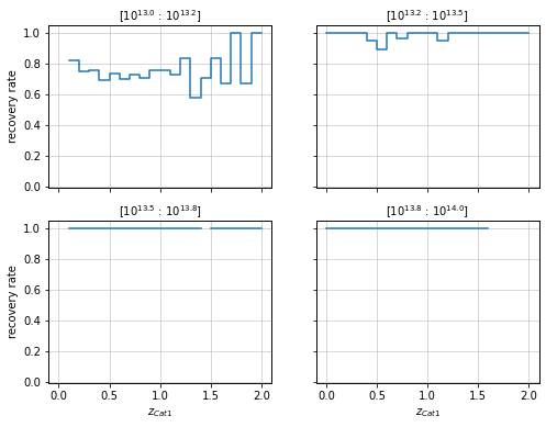
Panels plots
You can also have a panel for each bin:
zbins = np.linspace(0, 2, 21)
mbins = np.logspace(13, 14, 5)
info = recovery.plot_panel(c1, 'cross', zbins, mbins)
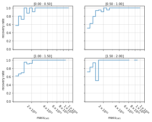
zbins = np.linspace(0, 2, 5)
mbins = np.logspace(13, 14, 20)
info = recovery.plot_panel(c1, 'cross', zbins, mbins, transpose=True)
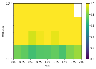
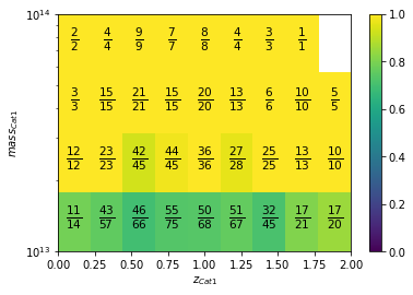
2D plots
zbins = np.linspace(0, 2, 10)
mbins = np.logspace(13, 14, 5)

info = recovery.plot2D(c1, 'cross', zbins, mbins)
plt.show()
info = recovery.plot2D(c1, 'cross', zbins, mbins,
                       add_num=True, num_kwargs={'fontsize':15})
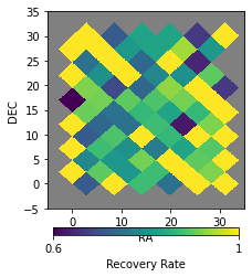
Sky plots
It is possible to plot the recovery rate by positions in the sky. It is done based on healpix pixelizations:
info = recovery.skyplot(c1, 'cross', nside=16, ra_lim=[-5, 35], dec_lim=[-5, 35])
/home/aguena/miniconda3/envs/clmmenv/lib/python3.9/site-packages/healpy/projaxes.py:920: MatplotlibDeprecationWarning: You are modifying the state of a globally registered colormap. In future versions, you will not be able to modify a registered colormap in-place. To remove this warning, you can make a copy of the colormap first. cmap = copy.copy(mpl.cm.get_cmap("viridis"))
  newcm.set_over(newcm(1.0))
/home/aguena/miniconda3/envs/clmmenv/lib/python3.9/site-packages/healpy/projaxes.py:921: MatplotlibDeprecationWarning: You are modifying the state of a globally registered colormap. In future versions, you will not be able to modify a registered colormap in-place. To remove this warning, you can make a copy of the colormap first. cmap = copy.copy(mpl.cm.get_cmap("viridis"))
  newcm.set_under(bgcolor)
/home/aguena/miniconda3/envs/clmmenv/lib/python3.9/site-packages/healpy/projaxes.py:922: MatplotlibDeprecationWarning: You are modifying the state of a globally registered colormap. In future versions, you will not be able to modify a registered colormap in-place. To remove this warning, you can make a copy of the colormap first. cmap = copy.copy(mpl.cm.get_cmap("viridis"))
  newcm.set_bad(badcolor)
/home/aguena/miniconda3/envs/clmmenv/lib/python3.9/site-packages/healpy/projaxes.py:202: MatplotlibDeprecationWarning: Passing parameters norm and vmin/vmax simultaneously is deprecated since 3.3 and will become an error two minor releases later. Please pass vmin/vmax directly to the norm when creating it.
  aximg = self.imshow(
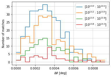
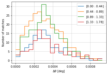
Distances of matching
Here we evaluate the distance between the cluster centers and their redshifts. These distances can be shown for all matched clusters, or in bins:
from clevar.match_metrics import distances
info = distances.central_position(
    c1, c2, 'cross', radial_bins=20, radial_bin_units='degrees')

info = distances.central_position(
    c1, c2, 'cross', radial_bins=20, radial_bin_units='degrees',
    quantity_bins='mass', bins=mbins, log_quantity=True)
info = distances.central_position(
    c1, c2, 'cross', radial_bins=20, radial_bin_units='degrees',
    quantity_bins='z', bins=zbins[::2], log_quantity=False)
info = distances.redshift(c1, c2, 'cross', redshift_bins=20, normalize='cat1')
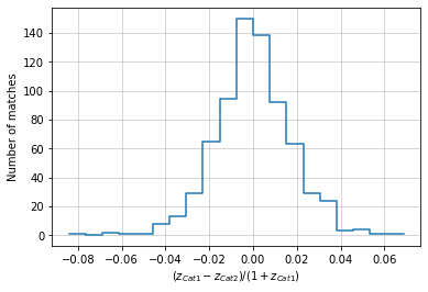
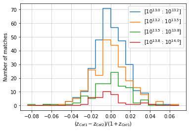
info = distances.redshift(
    c1, c2, 'cross', redshift_bins=20, normalize='cat1',
    quantity_bins='mass', bins=mbins, log_quantity=True)
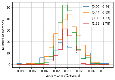
info = distances.redshift(
    c1, c2, 'cross', redshift_bins=20, normalize='cat1',
    quantity_bins='z', bins=zbins[::2], log_quantity=False)
The full information of the distances is outputed in a dictionary containing:
distances: values of distances.data: Binned data used in the plot. It has the sections:hist: Binned distances with (distance_bins, bin2). bins where no cluster was found have nan value.distance_bins: The bin edges for distances.bins2(optional): The bin edges along the second dimension.
info.keys()
dict_keys(['distances', 'data', 'ax'])
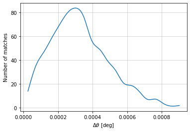
You can also smoothen the lines of the plot:
info = distances.central_position(
    c1, c2, 'cross', radial_bins=20, radial_bin_units='degrees',
    shape='line', plt_kwargs={'n_increase':3})
Scaling Relations
from clevar.match_metrics import scaling
Redshift plots
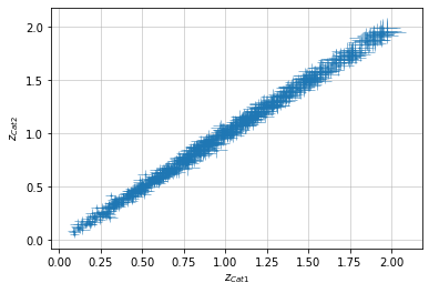
Simple plot
info = scaling.redshift(c1, c2, 'cross')
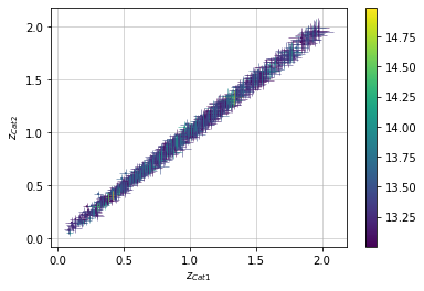
Color points by \(\log(M)\) value
info = scaling.redshift_masscolor(c1, c2, 'cross', add_err=True)
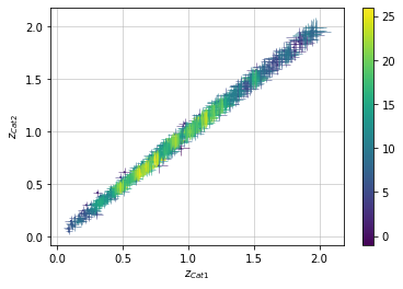
Color points by density at plot
info = scaling.redshift_density(c1, c2, 'cross', add_err=True)
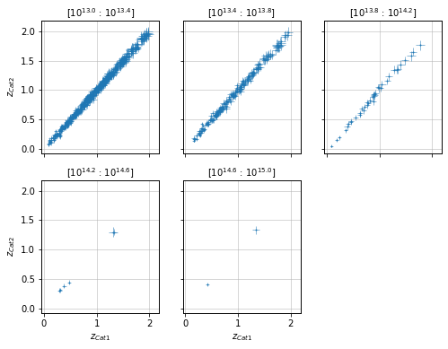
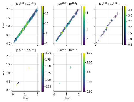
Split data into mass bins
info = scaling.redshift_masspanel(c1, c2, 'cross', add_err=True)
Split data into mass bins and color by density
info = scaling.redshift_density_masspanel(c1, c2, 'cross', add_err=True)
Evaluate metrics of the distribution
info = scaling.redshift_metrics(c1, c2, 'cross')
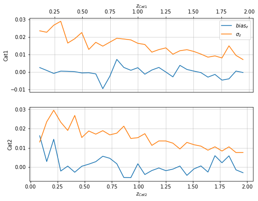
info = scaling.redshift_density_metrics(c1, c2, 'cross', ax_rotation=45)
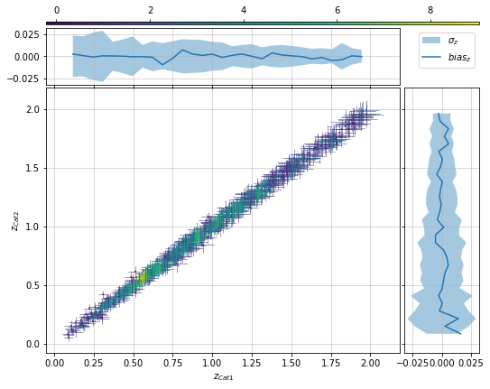
info = scaling.redshift_density_dist(c1, c2, 'cross', ax_rotation=45, add_err=False)
All of these functions with scatter plot can also fit a relation:
info = scaling.redshift_density_metrics(
    c1, c2, 'cross', ax_rotation=45,
    add_fit=True, fit_bins1=20)
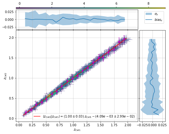
The full information of the scaling relation is outputed to a dictionay containing:
binned_data(optional): input data for fitting, with values:x: x values in fit (log of values if log=True).y: y values in fit (log of values if log=True).y_err: errorbar on y values (error_log if log=True).
fit(optional): fitting output dictionary, with values:pars: fitted parameter.cov: covariance of fitted parameters.func: fitting function with fitted parameter.func_plus: fitting function with fitted parameter plus 1x scatter.func_minus: fitting function with fitted parameter minus 1x scatter.func_scat: scatter of fited function.func_dist:P(y|x)- Probability of having y given a value for x, assumes normal distribution and uses scatter of the fitted function.func_scat_interp: interpolated scatter from data.func_dist_interp:P(y|x)using interpolated scatter.
plots(optional): additional plots:fit: fitted dataerrorbar: binned data
info['fit']['pars']
array([ 1.00479763, -0.00409297])
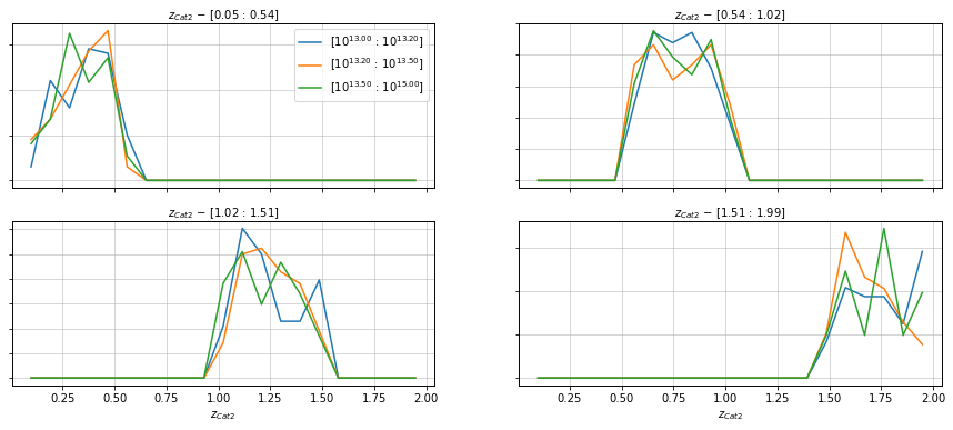
Evaluate the distribution
See how the distribution of mass happens in each bin for one of the catalogs
%%time
info = scaling.redshift_dist_self(
    c2, redshift_bins_dist=21,
    mass_bins=[10**13.0, 10**13.2, 10**13.5, 1e15],
    redshift_bins=4, shape='line',
    fig_kwargs={'figsize':(15, 6)})
CPU times: user 196 ms, sys: 161 ms, total: 357 ms
Wall time: 134 ms
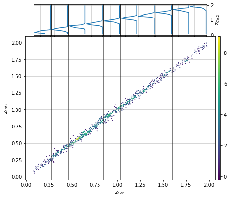
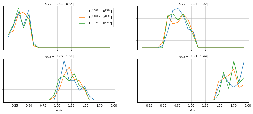
Compare with the distribution on the other catalog
%%time
info = scaling.redshift_dist(
    c1, c2, 'cross', redshift_bins_dist=21,
    mass_bins=[10**13.0, 10**13.2, 10**13.5, 1e15],
    redshift_bins=4, shape='line',
    fig_kwargs={'figsize':(15, 6)})
CPU times: user 231 ms, sys: 195 ms, total: 427 ms
Wall time: 173 ms
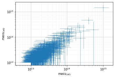
Mass plots
Simple plot
info = scaling.mass(c1, c2, 'cross', add_err=True)
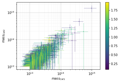
Color points by redshift value
info = scaling.mass_zcolor(c1, c2, 'cross', add_err=True)
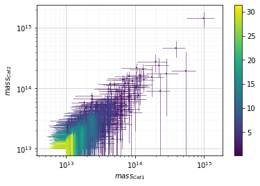
Color points by density at plot
info = scaling.mass_density(c1, c2, 'cross', add_err=True)
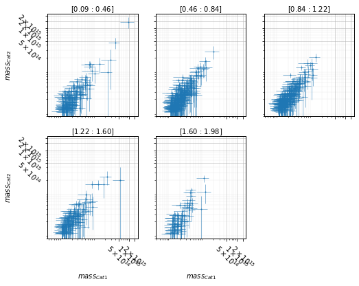
Split data into redshift bins
info = scaling.mass_zpanel(c1, c2, 'cross', add_err=True)
for ax in info['axes'].flatten():
    ax.set_ylim(.8e13, 2.2e15)
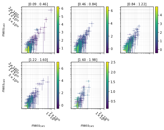
Split data into redshift bins and color by density
info = scaling.mass_density_zpanel(c1, c2, 'cross', add_err=True)
for ax in info['axes'].flatten():
    ax.set_ylim(.8e13, 2.2e15)
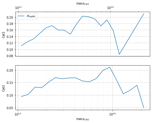
Evaluate metrics of the distribution
info = scaling.mass_metrics(c1, c2, 'cross')
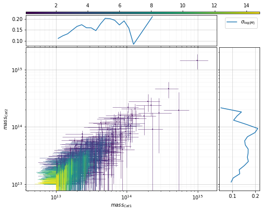
info = scaling.mass_density_metrics(c1, c2, 'cross', ax_rotation=45)
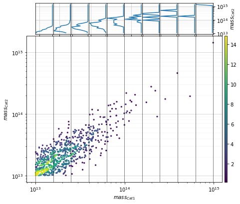
info = scaling.mass_density_dist(c1, c2, 'cross', ax_rotation=45,
                                 add_err=False, plt_kwargs={'s':5})
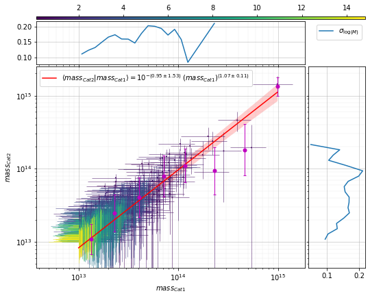
All of these functions with scatter plot can also fit a relation:
info = scaling.mass_density_metrics(
    c1, c2, 'cross', ax_rotation=45,
    add_fit=True, fit_bins1=8)
The full information of the scaling relation is outputed to a dictionay containing:
fit(optional): fitting output dictionary, with values:pars: fitted parameter.cov: covariance of fitted parameters.func: fitting function with fitted parameter.func_plus: fitting function with fitted parameter plus 1x scatter.func_minus: fitting function with fitted parameter minus 1x scatter.func_scat: scatter of fited function.func_chi: sqrt of chi_square(x, y) for the fitted function.
plots(optional): additional plots:fit: fitted dataerrorbar: binned data
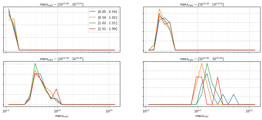
Evaluate the distribution
See how the distribution of mass happens in each bin for one of the catalogs
%%time
info = scaling.mass_dist_self(
    c2, mass_bins_dist=21,
    mass_bins=[10**13.0, 10**13.2, 10**13.5, 1e14, 1e15],
    redshift_bins=4, shape='line',
    fig_kwargs={'figsize':(15, 6)})
CPU times: user 224 ms, sys: 170 ms, total: 394 ms
Wall time: 158 ms
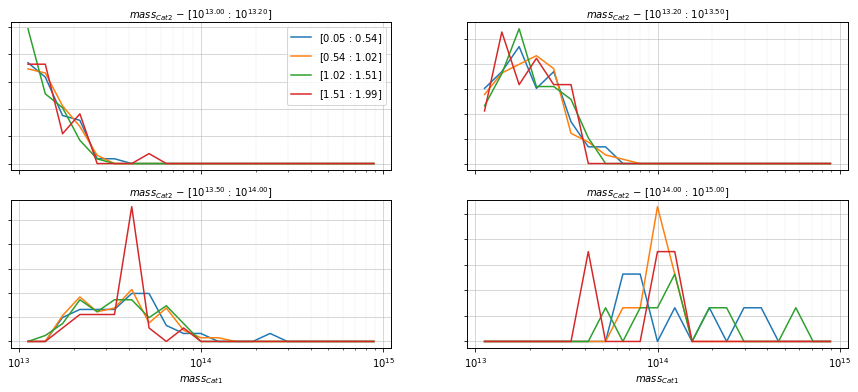
Compare with the distribution on the other catalog
%%time
info = scaling.mass_dist(
    c1, c2, 'cross', mass_bins_dist=21,
    mass_bins=[10**13.0, 10**13.2, 10**13.5, 1e14, 1e15],
    redshift_bins=4, shape='line',
    fig_kwargs={'figsize':(15, 6)})
CPU times: user 436 ms, sys: 175 ms, total: 611 ms
Wall time: 375 ms