Metrics of matching (advanced)
Example of the more functions to plot metrics of matching, using non-standard quantities of the catalogs
Table of Contents
1 Generate random data and add to catalog
2 Match catalogs
3 Recovery rate
3.1 Binned plot
3.2 Sky plots
4 Distances of matching
5 Scaling Relations
%load_ext autoreload
%autoreload 2
import numpy as np
import pylab as plt
Generate random data and add to catalog
# For reproducibility
np.random.seed(1)
from support import gen_cluster
input1, input2 = gen_cluster(ra_min=0, ra_max=30, dec_min=0, dec_max=30)
Initial number of clusters (logM>12.48): 2,740
Clusters in catalog1: 835
Clusters in catalog2: 928
from clevar import ClCatalog
c1 = ClCatalog('Cat1', ra=input1['RA'], dec=input1['DEC'], z=input1['Z'], mass=input1['MASS'],
            mass_err=input1['MASS_ERR'], z_err=input1['Z_ERR'])
c2 = ClCatalog('Cat2', ra=input2['RA'], dec=input2['DEC'], z=input2['Z'], mass=input2['MASS'],
            mass_err=input2['MASS_ERR'], z_err=input2['Z_ERR'])
# Format for nice display
for c in ('ra', 'dec', 'z', 'z_err'):
    c1[c].info.format = '.2f'
    c2[c].info.format = '.2f'
for c in ('mass', 'mass_err'):
    c1[c].info.format = '.2e'
    c2[c].info.format = '.2e'
/home/aguena/.local/lib/python3.9/site-packages/clevar-0.13.2-py3.9.egg/clevar/catalog.py:267: UserWarning: id column missing, additional one is being created.
  warnings.warn(
Match catalogs
from clevar.match import ProximityMatch
from clevar.cosmology import AstroPyCosmology

match_config = {
    'type': 'cross', # options are cross, cat1, cat2
    'which_radius': 'max', # Case of radius to be used, can be: cat1, cat2, min, max
    'preference': 'angular_proximity', # options are more_massive, angular_proximity or redshift_proximity
    'catalog1': {'delta_z':.2,
                'match_radius': '1 mpc'
                },
    'catalog2': {'delta_z':.2,
                'match_radius': '10 arcsec'
                }
}

cosmo = AstroPyCosmology()
mt = ProximityMatch()
mt.match_from_config(c1, c2, match_config, cosmo=cosmo)
## ClCatalog 1
## Prep mt_cols
* zmin|zmax from config value
* ang radius from set scale

## ClCatalog 2
## Prep mt_cols
* zmin|zmax from config value
* ang radius from set scale

## Multiple match (catalog 1)
Finding candidates (Cat1)
* 719/835 objects matched.

## Multiple match (catalog 2)
Finding candidates (Cat2)
* 721/928 objects matched.

## Finding unique matches of catalog 1
Unique Matches (Cat1)
* 719/835 objects matched.

## Finding unique matches of catalog 2
Unique Matches (Cat2)
* 720/928 objects matched.
Cross Matches (Cat1)
* 719/835 objects matched.
Cross Matches (Cat2)
* 719/928 objects matched.
Recovery rate
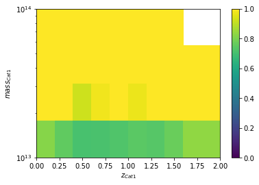
Compute recovery rates, in the main functions they are computed in mass and redshift bins. Here a more advanced use where different quantities can be used. There are several ways they can be displayed: - Single panel with multiple lines - Multiple panels - 2D color map
To use this, import the ClCatalogFuncs package from recovery. It
contains the functions: - plot - plot_panel - plot2D
There functions have the names of the columns as arguments, so you can use different columns available in the catalogs.
from clevar.match_metrics.recovery import ClCatalogFuncs as r_cf
zbins = np.linspace(0, 2, 11)
mbins = np.logspace(13, 14, 5)
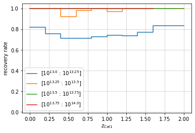
Binned plot
The recovery rates are shown as a function of col1 in col2 bins.
They can be displayed as a continuous line or with steps:
info = r_cf.plot(c1, col1='z', col2='mass', bins1=zbins, bins2=mbins,
        matching_type='cross', legend_format=lambda x: f'10^{{{np.log10(x)}}}')
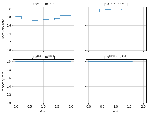
They can also be transposed to be shown as a function of mass in redshift bins.
info = r_cf.plot_panel(c1, col1='z', col2='mass', bins1=zbins, bins2=mbins,
        matching_type='cross', label_format=lambda x: f'10^{{{np.log10(x)}}}')
info = r_cf.plot2D(c1, col1='z', col2='mass', bins1=zbins, bins2=mbins,
        matching_type='cross', scale2='log')
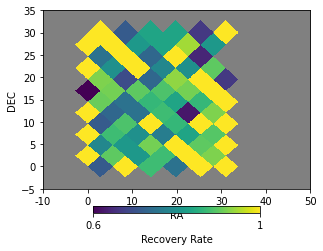
Sky plots
It is possible to plot the recovery rate by positions in the sky. It is done based on healpix pixelizations:
info = r_cf.skyplot(c1, matching_type='cross', nside=16, ra_lim=[-10, 50], dec_lim=[-5, 35])
/home/aguena/miniconda3/envs/clmmenv/lib/python3.9/site-packages/healpy/projaxes.py:920: MatplotlibDeprecationWarning: You are modifying the state of a globally registered colormap. In future versions, you will not be able to modify a registered colormap in-place. To remove this warning, you can make a copy of the colormap first. cmap = copy.copy(mpl.cm.get_cmap("viridis"))
  newcm.set_over(newcm(1.0))
/home/aguena/miniconda3/envs/clmmenv/lib/python3.9/site-packages/healpy/projaxes.py:921: MatplotlibDeprecationWarning: You are modifying the state of a globally registered colormap. In future versions, you will not be able to modify a registered colormap in-place. To remove this warning, you can make a copy of the colormap first. cmap = copy.copy(mpl.cm.get_cmap("viridis"))
  newcm.set_under(bgcolor)
/home/aguena/miniconda3/envs/clmmenv/lib/python3.9/site-packages/healpy/projaxes.py:922: MatplotlibDeprecationWarning: You are modifying the state of a globally registered colormap. In future versions, you will not be able to modify a registered colormap in-place. To remove this warning, you can make a copy of the colormap first. cmap = copy.copy(mpl.cm.get_cmap("viridis"))
  newcm.set_bad(badcolor)
/home/aguena/miniconda3/envs/clmmenv/lib/python3.9/site-packages/healpy/projaxes.py:202: MatplotlibDeprecationWarning: Passing parameters norm and vmin/vmax simultaneously is deprecated since 3.3 and will become an error two minor releases later. Please pass vmin/vmax directly to the norm when creating it.
  aximg = self.imshow(
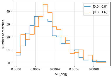
Distances of matching
The main functions in distances can already be binned along other
quantities of the catalog and do not require a more advanced use.
Nonetheless it also has a ClCatalogFuncs package and can be used
with the same formalism:
from clevar.match_metrics.distances import ClCatalogFuncs as d_cf
info = d_cf.central_position(c1, c2, 'cross', radial_bins=20, radial_bin_units='degrees',
                           col2='z', bins2=zbins[::4])
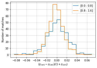
info = d_cf.redshift(c1, c2, 'cross', redshift_bins=20,
                   col2='z', bins2=zbins[::4], normalize='cat1')
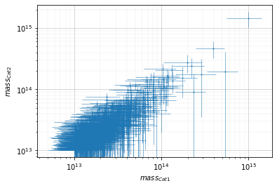
Scaling Relations
Here you will be able to evaluate the scaling relations of any two
quantities of the matched catalogs. Import the ClCatalogFuncs
package from scaling, the functions of this package are: - plot:
Scaling relation of a quantity - plot_color: Scaling relation of a
quantity with the colors based on a 2nd quantity - plot_density:
Scaling relation of a quantity with the colors based on density of
points - plot_panel: Scaling relation of a quantity divided in
panels based on a 2nd quantity - plot_color_panel: Scaling relation
of a quantity with the colors based on a 2nd quantity in panels based on
a 3rd quantity - plot_density_panel: Scaling relation of a quantity
with the colors based on density of points in panels based on a 2rd
quantity - plot_metrics: Metrics of quantity scaling relation. -
plot_density_metrics: Scaling relation of a quantity with the colors
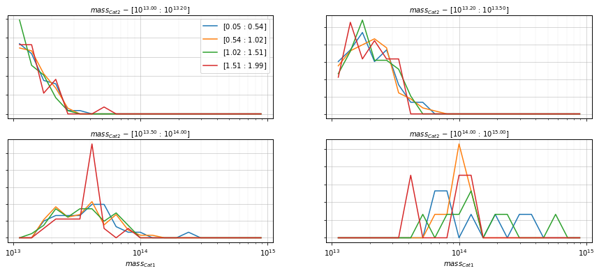
based on density of points with scatter and bias panels - plot_dist:
Distribution of a quantity, binned by other component in panels, and an
optional secondary component in lines. - plot_dist_self:
Distribution of a quantity, binned by the same quantity in panels, with
option for a second quantity in lines. Is is useful to compare with
plot_dist results.
take the name of the quantity to be binned:
from clevar.match_metrics.scaling import ClCatalogFuncs as s_cf
info = s_cf.plot(c1, c2, 'cross', col='mass', xscale='log', yscale='log')
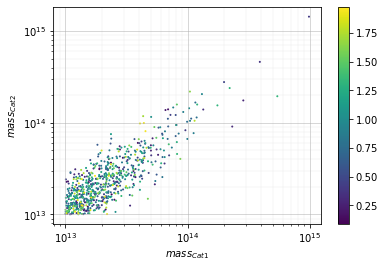
info = s_cf.plot(c1, c2, 'cross', col='mass', xscale='log', yscale='log',
                 col_color='z', add_err=False)
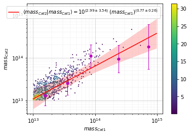
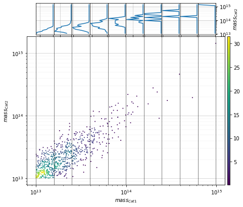
info = s_cf.plot_density(
    c1, c2, 'cross', col='mass',
    xscale='log', yscale='log', add_err=False,
    add_fit=True, fit_bins1=5, fit_log=True)
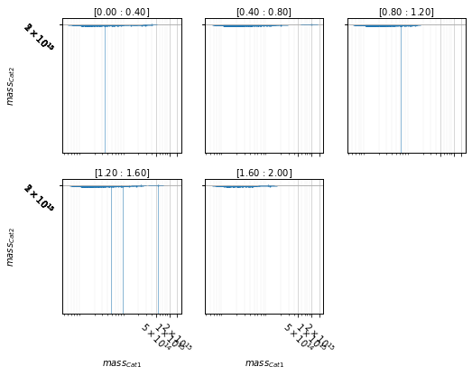
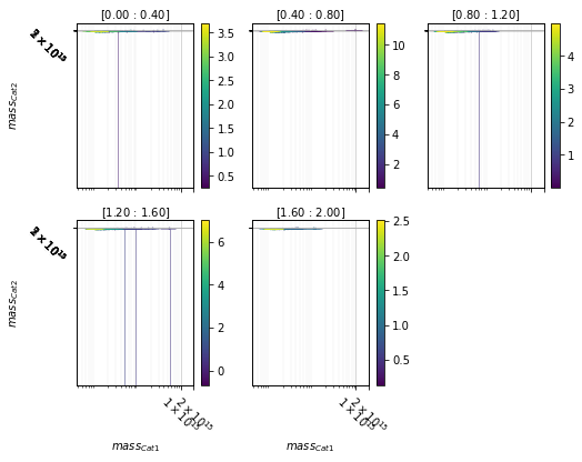
info = s_cf.plot_panel(
    c1, c2, 'cross', col='mass', xscale='log', yscale='log',
    col_panel='z', bins_panel=zbins[::2])
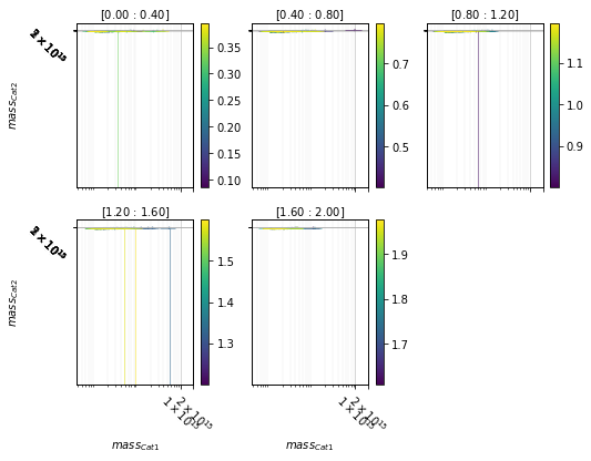
info = s_cf.plot_panel(
    c1, c2, 'cross', col='mass', xscale='log', yscale='log',
    col_panel='z', bins_panel=zbins[::2],
    col_color='z')
info = s_cf.plot_density_panel(
    c1, c2, 'cross', col='mass', xscale='log', yscale='log',
    col_panel='z', bins_panel=zbins[::2])
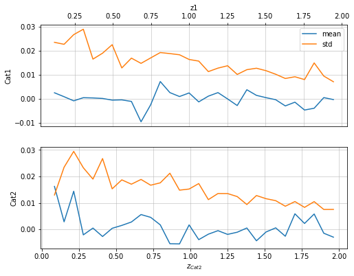
info = s_cf.plot_metrics(c1, c2, 'cross', col='z', mode='diff_z', label1='z1')
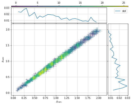
info = s_cf.plot_density_metrics(c1, c2, 'cross', col='z', metrics_mode='diff_z')
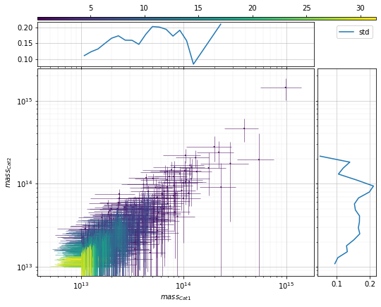
info = s_cf.plot_density_metrics(
    c1, c2, 'cross', col='mass', metrics_mode='log',
    scale1='log', scale2='log')
info = s_cf.plot_density_dist(
    c1, c2, 'cross', col='mass', metrics_mode='log',
    scale1='log', scale2='log', add_err=False)
zbins2 = np.linspace(0, 1.2, 7)[1:]
rbins2 = [1, 5.5, 25, 50, c2['mass'].max()]
bins1 = 10**np.histogram(np.log10(c1['mass']), 20)[1]
info = s_cf.plot_dist(
    c1, c2, 'cross', 'mass',
    bins1=21, bins2=[10**13.0, 10**13.2, 10**13.5, 1e14, 1e15],
    col_aux='z', bins_aux=4, shape='line',
    log_vals=True, fig_kwargs={'figsize':(15, 6)})