Hankel transforms¶

A Hankel transform converts a Fourier-space power spectrum into a real-space correlation statistic.

DSF provides three numerical backends through the HankelTransform class: fftlog, matrix_zeros, and matrix_direct.

The examples below demonstrate projected and spherical correlation functions, interpolation onto user-defined radial grids, and backend selection. Mathematical conventions and derivations are covered separately in the Hankel theory documentation.

Available backends¶

The backend argument selects the numerical implementation:

Backend	Supported operations	Practical considerations
`fftlog`	Projected and spherical correlation functions	Fastest option for most one-dimensional applications. Particularly useful for repeated evaluations.
`matrix_zeros`	Projected correlation functions and covariance matrices	Uses a Bessel-zero-based integration grid. Requires suitable numerical sampling and can exhibit small-scale ringing.
`matrix_direct`	Projected correlation functions and covariance matrices	Uses a direct matrix operator. Requires suitable wavenumber sampling and can exhibit some large-scale ringing.

All three backends are accessed through the same public class:

from dsf.hankel.hankel_transform import HankelTransform

hankel = HankelTransform(backend="fftlog")

FFTLog is the default backend, so HankelTransform() is equivalent to HankelTransform(backend="fftlog").

Projected correlation functions¶

Projected Hankel transforms are commonly used to convert angular or transverse Fourier-space spectra into real-space correlation functions.

The Bessel order determines the type of projected statistic. For example, order zero is used for isotropic projected correlations, while order two appears in tangential-shear calculations.

Here we use a smooth Gaussian spectrum in arbitrary units, with a dimensionless input grid, to illustrate the effect of changing the Bessel order.

import matplotlib.pyplot as plt
import numpy as np

from dsf import DSF_COLORS
from dsf.hankel.hankel_transform import HankelTransform

k = np.geomspace(1.0e-3, 1.0e2, 512)
spectrum = np.exp(-k**2)

hankel = HankelTransform(backend="fftlog")

r0, xi0 = hankel.projected_correlation(
    radial_input=k,
    spectrum=spectrum,
    order=0,
)

r2, xi2 = hankel.projected_correlation(
    radial_input=k,
    spectrum=spectrum,
    order=2,
)

fig, ax = plt.subplots()

ax.plot(
    r0,
    xi0,
    color=DSF_COLORS[0],
    label="Order 0",
)

ax.plot(
    r2,
    xi2,
    color=DSF_COLORS[1],
    label="Order 2",
)

ax.set_xscale("log")
ax.set_xlim(0.1, 10.0)
ax.set_xlabel(r"$R$")
ax.set_ylabel(r"Projected correlation")
ax.legend()

fig.tight_layout()
plt.show()

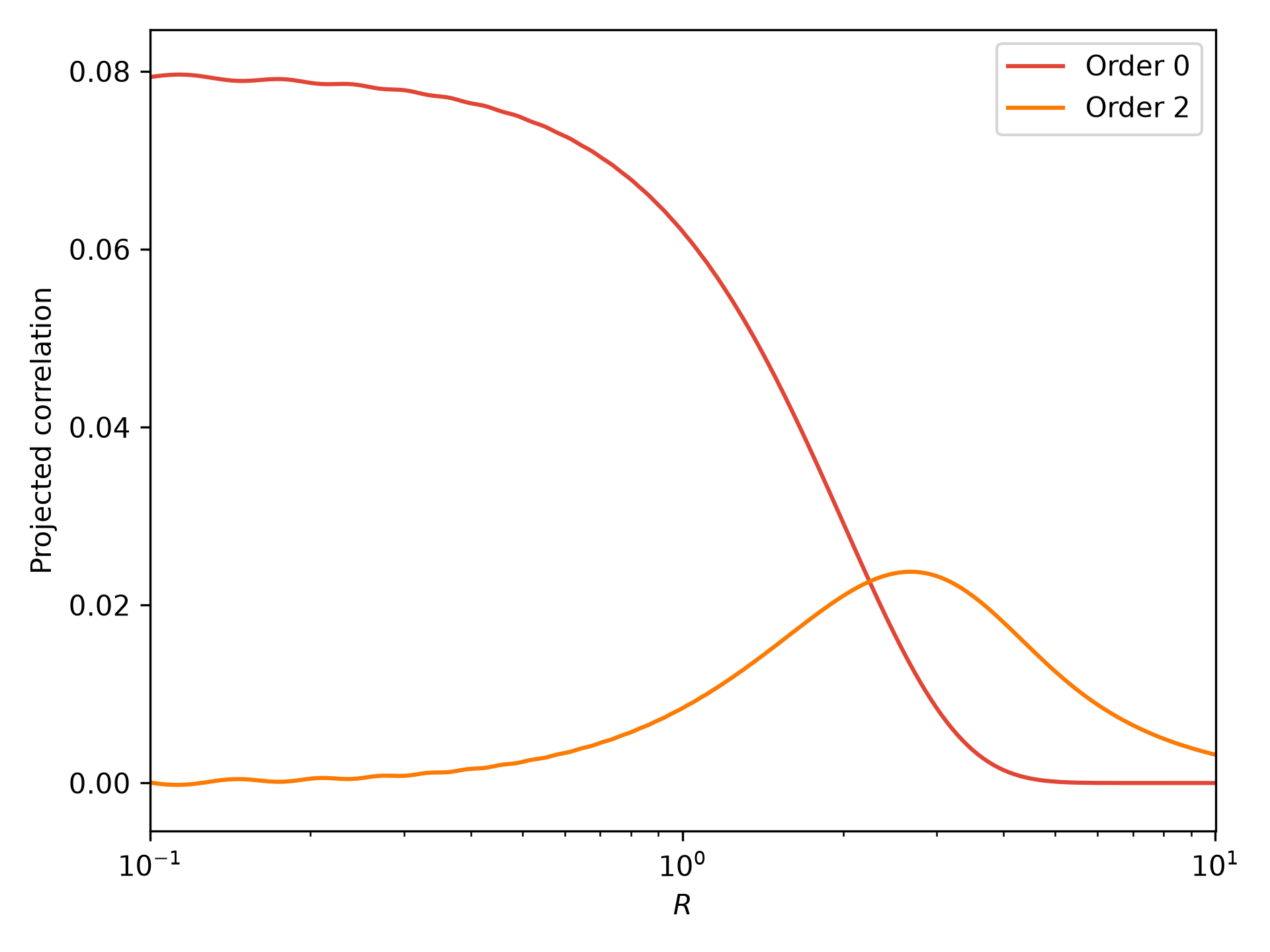
Both curves are obtained from the same input spectrum. The difference arises from the Bessel order used in the transformation.

The returned radial grid is determined internally by the selected backend and has inverse units relative to the input Fourier-space grid.

Interpolating onto a requested radial grid¶

In applications such as galaxy-galaxy lensing, predictions are often required at specific projected radii rather than on the internal transform grid.

DSF provides projected_correlation_interpolated for this purpose.

import matplotlib.pyplot as plt
import numpy as np

from dsf import DSF_COLORS
from dsf.hankel.hankel_transform import HankelTransform

k = np.geomspace(1.0e-3, 1.0e2, 512)
spectrum = np.exp(-k**2)

r_requested = np.geomspace(0.2, 10.0, 24)

hankel = HankelTransform(backend="fftlog")

r_full, xi_full = hankel.projected_correlation(
    radial_input=k,
    spectrum=spectrum,
    order=0,
)

r, xi = hankel.projected_correlation_interpolated(
    theta=r_requested,
    radial_input=k,
    spectrum=spectrum,
    order=0,
)

fig, ax = plt.subplots()

ax.plot(
    r_full,
    xi_full,
    color=DSF_COLORS[0],
    label="Internal transform grid",
)

ax.plot(
    r,
    xi,
    "o",
    color=DSF_COLORS[1],
    label="Requested radial grid",
)

ax.set_xscale("log")
ax.set_xlim(0.1, 12.0)
ax.set_xlabel(r"$R$")
ax.set_ylabel(r"Projected correlation")
ax.legend()

fig.tight_layout()
plt.show()

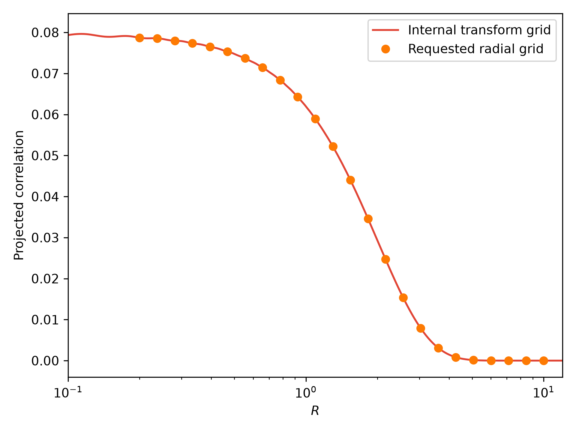
The interpolated method returns the requested radial coordinates together with the corresponding correlation values. This is convenient when constructing data vectors on a fixed radial grid.

The default interpolation uses linear spacing. Logarithmic interpolation is also available through grid_spacing="log" when the interpolated values are strictly positive.

Spherical correlation functions¶

DSF also supports spherical Hankel transforms, which convert three-dimensional power spectra into real-space correlation functions.

The spherical interface is available through spherical_correlation and spherical_correlation_interpolated.

The following example uses a Gaussian spectrum in arbitrary units.

import matplotlib.pyplot as plt
import numpy as np

from dsf import DSF_COLORS
from dsf.hankel.hankel_transform import HankelTransform

k = np.geomspace(1.0e-3, 1.0e2, 512)
pk = np.exp(-k**2)

hankel = HankelTransform(backend="fftlog")

r, xi = hankel.spherical_correlation(
    k_pk=k,
    pk=pk,
    order=0,
)

fig, ax = plt.subplots()

ax.plot(
    r,
    xi,
    color=DSF_COLORS[0],
)

ax.set_xscale("log")
ax.set_xlim(0.1, 10.0)
ax.set_xlabel(r"$r$")
ax.set_ylabel(r"$\xi(r)$")

fig.tight_layout()
plt.show()

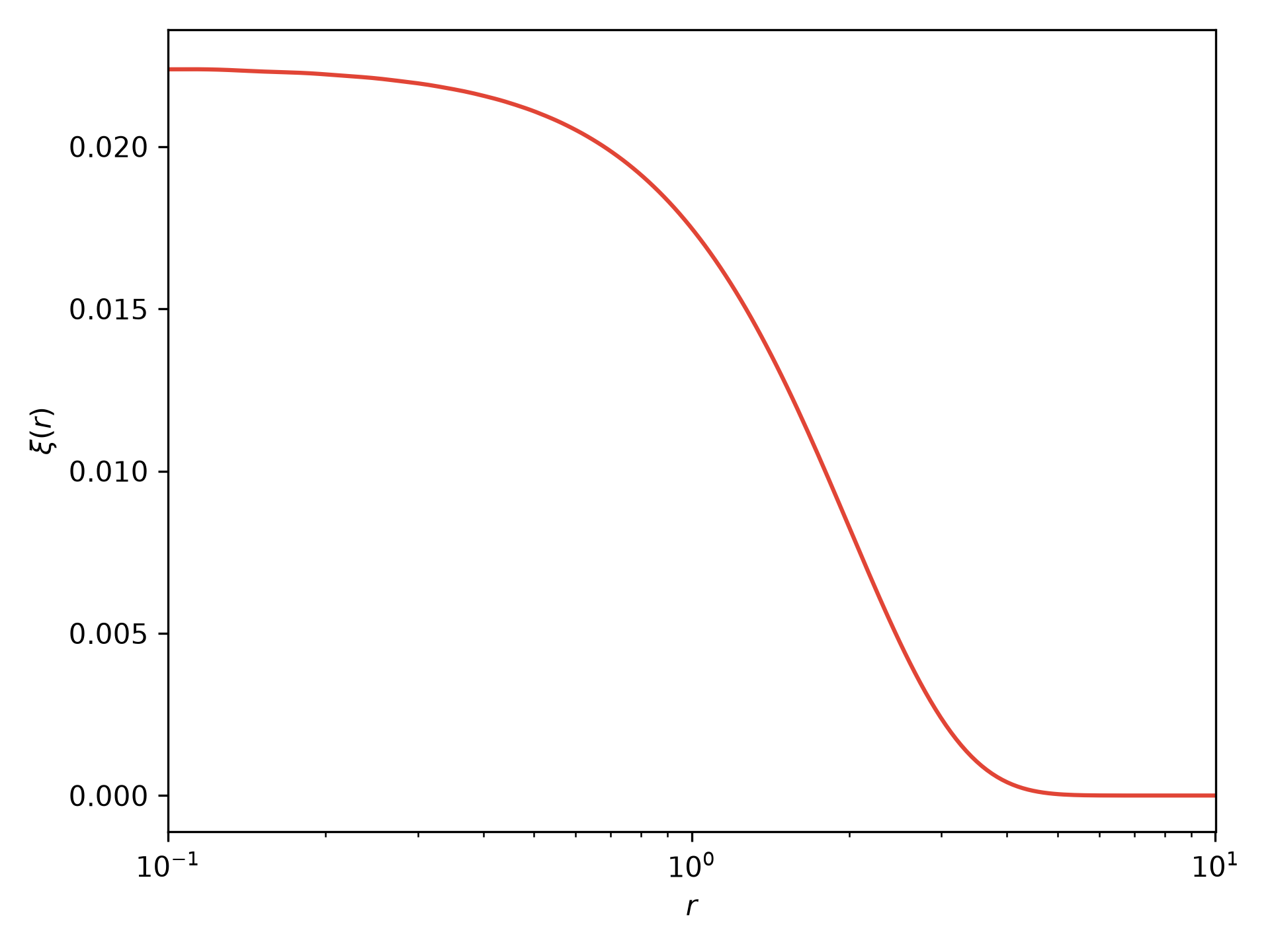
Unlike the projected transform, the spherical transform uses spherical Bessel functions and the three-dimensional Fourier-space integration measure.

For a power spectrum in units of \(\mathrm{Mpc}^3\) and wavenumbers in \(\mathrm{Mpc}^{-1}\), the resulting correlation function is dimensionless.

Choosing a backend¶

FFTLog is generally the preferred choice for one-dimensional correlation functions. The matrix backends additionally support projected covariance calculations, with different numerical sampling requirements.

For supported backends, covariance-related methods include projected_covariance, bin_radial_matrix, correlation_matrix, and diagonal_error.

See the covariance examples for their use in the DSF covariance pipeline.