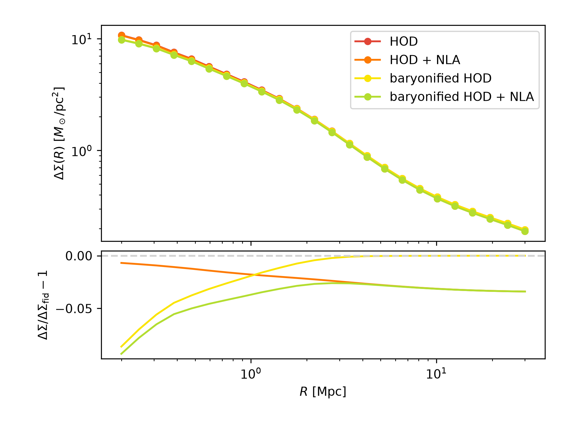
 Systematics modelling
DSF supports different physical ingredients through the pk2d_func
argument of DeltaSigmaCalculator. The examples below compare HOD,
intrinsic alignment, and baryonified power-spectrum models, and illustrate
a toy additive magnification bias contribution at the data-vector level.
All examples use the same projected-radius grid and lens redshift so that changes in the predicted \(\Delta\Sigma(R)\) can be compared directly. Each lower panel shows the fractional difference from the HOD baseline, \((\Delta\Sigma_{\rm model}-\Delta\Sigma_{\rm base})/\Delta\Sigma_{\rm base}\). These fractions require a nonzero baseline at the plotted radii. For a basic calculation, see Data vector.
Comparing physical models
The pk2d_func argument can be swapped to test different physical model
ingredients without changing the data-vector call.
import matplotlib.pyplot as plt
import numpy as np

from dsf import DSF_COLORS
from dsf.data_vector.delta_sigma_builder import DeltaSigmaCalculator
from dsf.modelling.cosmology import make_ccl_cosmology
from dsf.modelling.hod import pk2d_hod
from dsf.modelling.baryons import pk2d_hod_baryonified
from dsf.modelling.combinations import (
    pk2d_hod_with_nla,
    pk2d_hod_baryonified_with_nla,
)

cosmo = make_ccl_cosmology(
    transfer_function="eisenstein_hu",
    matter_power_spectrum="halofit",
)

r = np.geomspace(0.2, 30.0, 24)
z_lens = 0.55
a_lens = 1.0 / (1.0 + z_lens)

k_array = np.geomspace(1.0e-3, 30.0, 64)
a_array = np.linspace(0.3, 1.0, 16)

model_builders = {
    "HOD": lambda cosmo: pk2d_hod(
        cosmo,
        k_array=k_array,
        a_array=a_array,
    )["pk_deltasigma"],
    "HOD + NLA": lambda cosmo: pk2d_hod_with_nla(
        cosmo,
        k_array=k_array,
        a_array=a_array,
        A_IA=5.0,
        a_bias=a_lens,
    )["pk_deltasigma"],
    "baryonified HOD": lambda cosmo: pk2d_hod_baryonified(
        cosmo,
        k_array=k_array,
        a_array=a_array,
        f_c=0.8,
    )["pk_deltasigma"],
    "baryonified HOD + NLA": lambda cosmo: pk2d_hod_baryonified_with_nla(
        cosmo,
        k_array=k_array,
        a_array=a_array,
        f_c=0.8,
        A_IA=5.0,
        a_bias=a_lens,
    )["pk_deltasigma"],
}

colors = DSF_COLORS[:len(model_builders)]

fig, (ax, ax_res) = plt.subplots(
    2,
    1,
    sharex=True,
    gridspec_kw={"height_ratios": [3.0, 1.5], "hspace": 0.06},
)

curves = {}

for color, (label, builder) in zip(colors, model_builders.items()):
    calculator = DeltaSigmaCalculator(pk2d_func=builder)

    curves[label] = calculator.delta_sigma(
        r=r,
        a=a_lens,
        cosmo=cosmo,
    )

    ax.plot(
        r,
        curves[label],
        color=color,
        marker="o",
        markersize=5,
        label=label,
    )

baseline = curves["HOD"]

for color, (label, curve) in zip(colors[1:], list(curves.items())[1:]):
    ax_res.plot(
        r,
        (curve - baseline) / baseline,
        color=color,
    )

ax.set_xscale("log")
ax.set_yscale("log")
ax.set_ylabel(r"$\Delta\Sigma(R)\ [M_\odot / {\rm pc}^2]$")
ax.legend()

ax_res.axhline(0.0, color="lightgray", linestyle="--")
ax_res.set_xscale("log")
ax_res.set_ylabel(r"$\Delta\Sigma/\Delta\Sigma_{\rm fid}-1$")
ax_res.set_xlabel(r"$R\ [{\rm Mpc}]$")

fig.subplots_adjust(left=0.18, right=0.97, bottom=0.15, top=0.94)

plt.show()
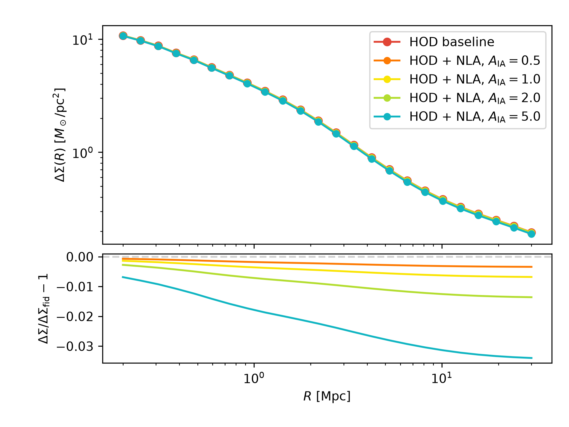
Intrinsic alignments
Intrinsic alignments arise when galaxy shapes are correlated with the
surrounding tidal field, introducing correlations that can contaminate
weak lensing measurements. The nonlinear linear alignment (NLA) model describes
this contribution through the amplitude A_IA, varied below while
keeping the HOD baseline fixed.
import matplotlib.pyplot as plt
import numpy as np

from dsf import DSF_COLORS
from dsf.data_vector.delta_sigma_builder import DeltaSigmaCalculator
from dsf.modelling.cosmology import make_ccl_cosmology
from dsf.modelling.hod import pk2d_hod
from dsf.modelling.combinations import pk2d_hod_with_nla


cosmo = make_ccl_cosmology(
    transfer_function="eisenstein_hu",
    matter_power_spectrum="halofit",
)

r = np.geomspace(0.2, 30.0, 24)
z_lens = 0.55
a_lens = 1.0 / (1.0 + z_lens)

k_array = np.geomspace(1.0e-3, 30.0, 64)
a_array = np.linspace(0.3, 1.0, 16)


def pk2d_baseline(*, cosmo):
    return pk2d_hod(
        cosmo,
        k_array=k_array,
        a_array=a_array,
    )["pk_deltasigma"]


baseline_calculator = DeltaSigmaCalculator(pk2d_func=pk2d_baseline)

delta_sigma_baseline = baseline_calculator.delta_sigma(
    r=r,
    a=a_lens,
    cosmo=cosmo,
)

ia_amplitudes = [0.5, 1.0, 2.0, 5.0]

colors = DSF_COLORS[:len(ia_amplitudes) + 1]

fig, (ax, ax_res) = plt.subplots(
    2,
    1,
    sharex=True,
    gridspec_kw={"height_ratios": [3.0, 1.5], "hspace": 0.06},
)

ax.plot(
    r,
    delta_sigma_baseline,
    color=colors[0],
    marker="o",
    markersize=6,
    label="HOD baseline",
)

for color, A_IA in zip(colors[1:], ia_amplitudes):

    def pk2d_func(*, cosmo, A_IA=A_IA):
        return pk2d_hod_with_nla(
            cosmo,
            k_array=k_array,
            a_array=a_array,
            A_IA=A_IA,
            a_bias=a_lens,
        )["pk_deltasigma"]

    calculator = DeltaSigmaCalculator(pk2d_func=pk2d_func)

    delta_sigma_ia = calculator.delta_sigma(
        r=r,
        a=a_lens,
        cosmo=cosmo,
    )

    ax.plot(
        r,
        delta_sigma_ia,
        color=color,
        marker="o",
        markersize=5,
        label=rf"HOD + NLA, $A_{{\rm IA}}={A_IA:.1f}$",
    )

    ax_res.plot(
        r,
        (delta_sigma_ia - delta_sigma_baseline) / delta_sigma_baseline,
        color=color,
    )

ax.set_xscale("log")
ax.set_yscale("log")
ax.set_ylabel(r"$\Delta\Sigma(R)\ [M_\odot / {\rm pc}^2]$")
ax.legend()

ax_res.axhline(0.0, color="lightgray", linestyle="--")
ax_res.set_xscale("log")
ax_res.set_ylabel(r"$\Delta\Sigma/\Delta\Sigma_{\rm fid}-1$")
ax_res.set_xlabel(r"$R\ [{\rm Mpc}]$")

fig.subplots_adjust(left=0.18, right=0.97, bottom=0.15, top=0.94)

plt.show()
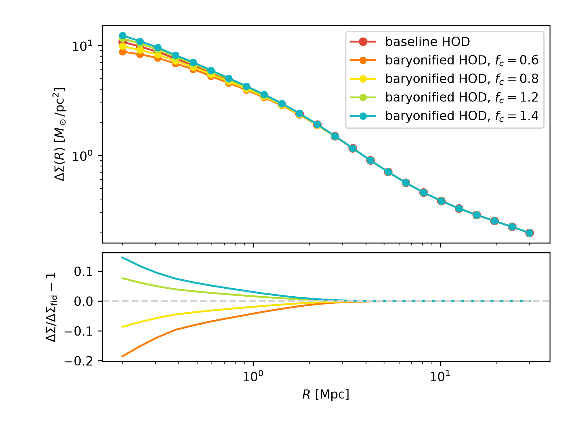
Baryonic effects
Baryonic processes can redistribute matter within halos and modify the
small-scale matter distribution. DSF approximates these effects by rescaling
the halo concentration-mass relation through f_c, with four values
compared against the standard HOD prediction.
import matplotlib.pyplot as plt
import numpy as np

from dsf import DSF_COLORS
from dsf.data_vector.delta_sigma_builder import DeltaSigmaCalculator
from dsf.modelling.cosmology import make_ccl_cosmology
from dsf.modelling.hod import pk2d_hod
from dsf.modelling.baryons import pk2d_hod_baryonified


cosmo = make_ccl_cosmology(
    transfer_function="eisenstein_hu",
    matter_power_spectrum="halofit",
)

r = np.geomspace(0.2, 30.0, 24)

z_lens = 0.55
a_lens = 1.0 / (1.0 + z_lens)

k_array = np.geomspace(1.0e-3, 30.0, 64)
a_array = np.linspace(0.3, 1.0, 16)


def pk2d_baseline(*, cosmo):
    return pk2d_hod(
        cosmo,
        k_array=k_array,
        a_array=a_array,
    )["pk_deltasigma"]


baseline_calculator = DeltaSigmaCalculator(
    pk2d_func=pk2d_baseline,
)

delta_sigma_baseline = baseline_calculator.delta_sigma(
    r=r,
    a=a_lens,
    cosmo=cosmo,
)

baryon_levels = [0.6, 0.8, 1.2, 1.4]

colors = DSF_COLORS[:len(baryon_levels) + 1]

fig, (ax, ax_res) = plt.subplots(
    2,
    1,
    sharex=True,
    gridspec_kw={"height_ratios": [3.0, 1.5], "hspace": 0.06},
)

ax.plot(
    r,
    delta_sigma_baseline,
    color=colors[0],
    marker="o",
    markersize=6,
    label="baseline HOD",
)

for color, f_c in zip(colors[1:], baryon_levels):

    def pk2d_func(*, cosmo, f_c=f_c):
        return pk2d_hod_baryonified(
            cosmo,
            k_array=k_array,
            a_array=a_array,
            f_c=f_c,
        )["pk_deltasigma"]

    calculator = DeltaSigmaCalculator(pk2d_func=pk2d_func)

    delta_sigma_baryons = calculator.delta_sigma(
        r=r,
        a=a_lens,
        cosmo=cosmo,
    )

    ax.plot(
        r,
        delta_sigma_baryons,
        color=color,
        marker="o",
        markersize=5,
        label=rf"baryonified HOD, $f_c={f_c:.1f}$",
    )

    ax_res.plot(
        r,
        (delta_sigma_baryons - delta_sigma_baseline) / delta_sigma_baseline,
        color=color,
    )

ax.set_xscale("log")
ax.set_yscale("log")
ax.set_ylabel(r"$\Delta\Sigma(R)\ [M_\odot / {\rm pc}^2]$")
ax.legend()

ax_res.axhline(
    0.0,
    color="lightgray",
    linestyle="--",
)

ax_res.set_xscale("log")
ax_res.set_ylabel(r"$\Delta\Sigma/\Delta\Sigma_{\rm fid}-1$")
ax_res.set_xlabel(r"$R\ [{\rm Mpc}]$")

fig.subplots_adjust(
    left=0.18,
    right=0.97,
    bottom=0.15,
    top=0.94,
)

plt.show()
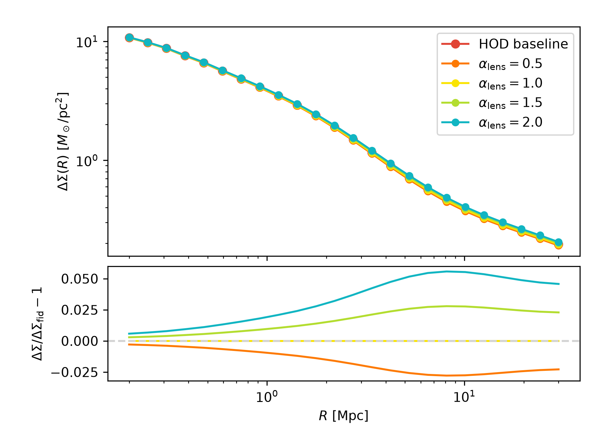
Magnification bias
Gravitational lensing changes the observed number density of lens galaxies
through flux magnification and area distortion, introducing an additional
contribution to galaxy-galaxy lensing. DSF computes the lens-magnification
correction using the nonlinear matter power spectrum and lensing geometry,
with an amplitude proportional to alpha_lens - 1.
The example compares four magnification slopes against the unmodified HOD prediction. The magnification-contaminated signal is constructed by adding the correction to the baseline prediction. The correction can subsequently be subtracted from an observed signal.
import matplotlib.pyplot as plt
import numpy as np

from dsf import DSF_COLORS
from dsf.data_vector.delta_sigma_builder import DeltaSigmaCalculator
from dsf.modelling import (
    make_ccl_cosmology,
    pk2d_hod,
    delta_sigma_lens_mag_correction,
)

cosmo = make_ccl_cosmology(
    transfer_function="eisenstein_hu",
    matter_power_spectrum="halofit",
)

r = np.geomspace(0.2, 30.0, 24)

z_lens = 0.55
z_source = 1.0

a_lens = 1.0 / (1.0 + z_lens)
a_source = 1.0 / (1.0 + z_source)

k_array = np.geomspace(1.0e-3, 30.0, 64)
a_array = np.linspace(0.3, 1.0, 16)

def pk2d_func(*, cosmo):
    return pk2d_hod(
        cosmo,
        k_array=k_array,
        a_array=a_array,
    )["pk_deltasigma"]

calculator = DeltaSigmaCalculator(pk2d_func=pk2d_func)

delta_sigma_baseline = calculator.delta_sigma(
    r=r,
    a=a_lens,
    cosmo=cosmo,
)

# Compute once at alpha_lens = 2, where alpha_lens - 1 = 1.
correction_unit = delta_sigma_lens_mag_correction(
    r=r,
    a_lens=a_lens,
    a_source=a_source,
    cosmo=cosmo,
    alpha_lens=2.0,
)

alpha_values = [0.5, 1.0, 1.5, 2.0]
colors = DSF_COLORS[:len(alpha_values) + 1]

fig, (ax, ax_res) = plt.subplots(
    2,
    1,
    sharex=True,
    gridspec_kw={"height_ratios": [3.0, 1.5], "hspace": 0.06},
)

ax.plot(
    r,
    delta_sigma_baseline,
    color=colors[0],
    marker="o",
    markersize=6,
    label="HOD baseline",
)

for color, alpha_lens in zip(colors[1:], alpha_values):
    correction = (alpha_lens - 1.0) * correction_unit
    delta_sigma_modified = delta_sigma_baseline + correction

    ax.plot(
        r,
        delta_sigma_modified,
        color=color,
        marker="o",
        markersize=5,
        label=rf"$\alpha_{{\rm lens}}={alpha_lens:.1f}$",
    )

    ax_res.plot(
        r,
        correction / delta_sigma_baseline,
        color=color,
    )

ax.set_xscale("log")
ax.set_yscale("log")
ax.set_ylabel(r"$\Delta\Sigma(R)\ [M_\odot / {\rm pc}^2]$")
ax.legend()

ax_res.axhline(0.0, color="lightgray", linestyle="--")
ax_res.set_xscale("log")
ax_res.set_ylabel(r"$\Delta\Sigma/\Delta\Sigma_{\rm fid}-1$")
ax_res.set_xlabel(r"$R\ [{\rm Mpc}]$")

fig.subplots_adjust(left=0.18, right=0.97, bottom=0.15, top=0.94)

plt.show()