DeltaSigma data vector
This example shows how to compute a minimal \(\Delta\Sigma(R)\) data vector with DSF.
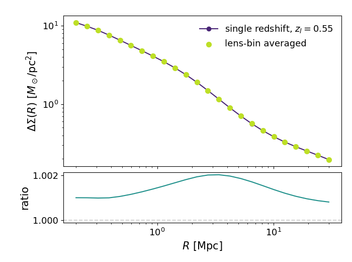
We use a small projected-radius grid, define a simple power-spectrum-backed profile model, evaluate \(\Delta\Sigma(R)\) at one lens redshift, and then compare it to a toy lens-bin-averaged signal.
This example only computes the data vector. It does not include covariance.
Minimal example
import cmasher as cmr
import matplotlib.pyplot as plt
import numpy as np

from dsf.data_vector.delta_sigma_builder import DeltaSigmaCalculator
from dsf.modelling import make_ccl_cosmology, pk2d_hod


cosmo = make_ccl_cosmology(
    transfer_function="eisenstein_hu",
    matter_power_spectrum="halofit",
)

r = np.geomspace(0.2, 30.0, 24)

z_lens = 0.55
a_lens = 1.0 / (1.0 + z_lens)

k_array = np.geomspace(1.0e-3, 30.0, 64)
a_array = np.linspace(0.3, 1.0, 16)


def pk2d_func(*, cosmo):
    return pk2d_hod(
        cosmo,
        k_array=k_array,
        a_array=a_array,
    )


calculator = DeltaSigmaCalculator(pk2d_func=pk2d_func)

delta_sigma = calculator.delta_sigma(
    r=r,
    a=a_lens,
    cosmo=cosmo,
)

z = np.linspace(0.45, 0.65, 9)
n_z = np.exp(-0.5 * ((z - z_lens) / 0.05) ** 2)

delta_sigma_bin = calculator.delta_sigma_lens_bin(
    r=r,
    lens_dndz=(z, n_z),
    cosmo=cosmo,
    z_min=0.45,
    z_max=0.65,
)

ratio = delta_sigma_bin / delta_sigma

colors = cmr.take_cmap_colors(
    "viridis",
    3,
    cmap_range=(0.10, 0.90),
    return_fmt="hex",
)

fig, (ax, ax_res) = plt.subplots(
    2,
    1,
    figsize=(7.0, 5.2),
    sharex=True,
    gridspec_kw={"height_ratios": [3.0, 1.0], "hspace": 0.06},
)

ax.plot(
    r,
    delta_sigma,
    color=colors[0],
    marker="o",
    markersize=6,
    label=rf"single redshift, $z_l={z_lens:.2f}$",
)

ax.scatter(
    r,
    delta_sigma_bin,
    color=colors[2],
    s=50,
    label="lens-bin averaged",
    zorder=3,
)

ax.set_xscale("log")
ax.set_yscale("log")

ax.set_ylabel(r"$\Delta\Sigma(R)\ [M_\odot / {\rm pc}^2]$", fontsize=15)
ax.tick_params(axis="both", which="major", labelsize=13)
ax.tick_params(axis="both", which="minor", labelsize=11)
ax.legend(fontsize=13, frameon=False)

ax_res.axhline(1.0, color="lightgray", linewidth=1.4, linestyle="--")
ax_res.plot(
    r,
    ratio,
    color=colors[1],
)

ax_res.set_xscale("log")
ax_res.set_ylabel("ratio", fontsize=15)
ax_res.set_xlabel(r"$R\ [{\rm Mpc}]$", fontsize=15)
ax_res.tick_params(axis="both", which="major", labelsize=13)
ax_res.tick_params(axis="both", which="minor", labelsize=11)

fig.subplots_adjust(left=0.18, right=0.97, bottom=0.15, top=0.94)

plt.show()
Model variants
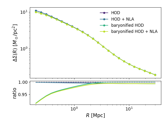
The pk2d_func argument can be swapped to test different physical model
ingredients without changing the data-vector call.
import cmasher as cmr
import matplotlib.pyplot as plt
import numpy as np

from dsf.data_vector.delta_sigma_builder import DeltaSigmaCalculator
from dsf.modelling import (
    make_ccl_cosmology,
    pk2d_hod,
    pk2d_hod_with_nla,
    pk2d_hod_baryonified,
    pk2d_hod_baryonified_with_nla,
)

cosmo = make_ccl_cosmology(
    transfer_function="eisenstein_hu",
    matter_power_spectrum="halofit",
)

r = np.geomspace(0.2, 30.0, 24)
z_lens = 0.55
a_lens = 1.0 / (1.0 + z_lens)

k_array = np.geomspace(1.0e-3, 30.0, 64)
a_array = np.linspace(0.3, 1.0, 16)

model_builders = {
    "HOD": lambda cosmo: pk2d_hod(
        cosmo,
        k_array=k_array,
        a_array=a_array,
    ),
    "HOD + NLA": lambda cosmo: pk2d_hod_with_nla(
        cosmo,
        k_array=k_array,
        a_array=a_array,
        A_IA=1.0,
        a_bias=a_lens,
    ),
    "baryonified HOD": lambda cosmo: pk2d_hod_baryonified(
        cosmo,
        k_array=k_array,
        a_array=a_array,
        f_c=0.8,
    ),
    "baryonified HOD + NLA": lambda cosmo: pk2d_hod_baryonified_with_nla(
        cosmo,
        k_array=k_array,
        a_array=a_array,
        f_c=0.8,
        A_IA=1.0,
        a_bias=a_lens,
    ),
}

colors = cmr.take_cmap_colors(
    "viridis",
    len(model_builders),
    cmap_range=(0.10, 0.90),
    return_fmt="hex",
)

fig, (ax, ax_res) = plt.subplots(
    2,
    1,
    figsize=(7.0, 5.2),
    sharex=True,
    gridspec_kw={"height_ratios": [3.0, 1.0], "hspace": 0.06},
)

curves = {}

for color, (label, builder) in zip(colors, model_builders.items()):
    calculator = DeltaSigmaCalculator(pk2d_func=builder)

    curves[label] = calculator.delta_sigma(
        r=r,
        a=a_lens,
        cosmo=cosmo,
    )

    ax.plot(
        r,
        curves[label],
        color=color,
        marker="o",
        markersize=5,
        label=label,
    )

baseline = curves["HOD"]

for color, (label, curve) in zip(colors, curves.items()):
    ax_res.plot(
        r,
        curve / baseline,
        color=color,
        linewidth=2.0,
    )

ax.set_xscale("log")
ax.set_yscale("log")
ax.set_ylabel(r"$\Delta\Sigma(R)\ [M_\odot / {\rm pc}^2]$", fontsize=15)
ax.tick_params(axis="both", which="major", labelsize=13)
ax.tick_params(axis="both", which="minor", labelsize=11)
ax.legend(fontsize=12, frameon=False)

ax_res.axhline(1.0, color="lightgray", linewidth=1.4, linestyle="--")
ax_res.set_xscale("log")
ax_res.set_ylabel("ratio", fontsize=15)
ax_res.set_xlabel(r"$R\ [{\rm Mpc}]$", fontsize=15)
ax_res.tick_params(axis="both", which="major", labelsize=13)
ax_res.tick_params(axis="both", which="minor", labelsize=11)

fig.subplots_adjust(left=0.18, right=0.97, bottom=0.15, top=0.94)

plt.show()
Magnification bias additive term
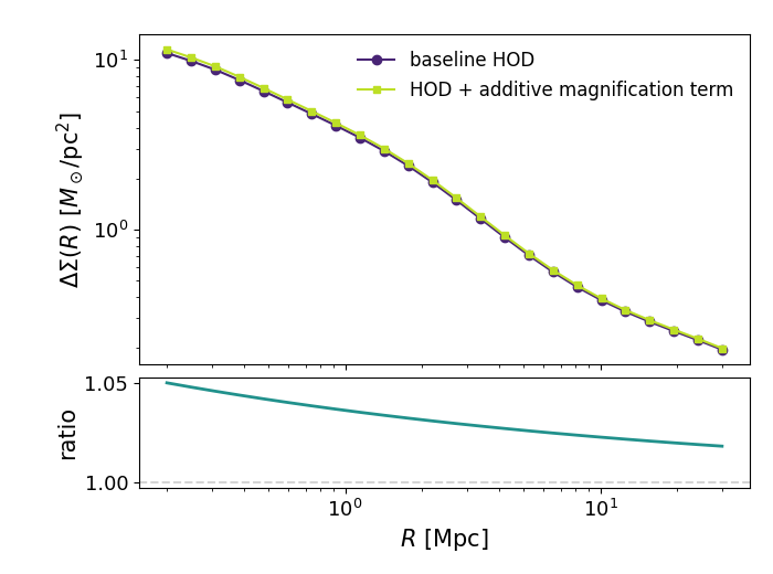
Magnification bias enters as an additive contribution at the
\(\Delta\Sigma\) level rather than as part of the Pk2D model. This
means it can be added after the baseline data vector has been evaluated.
import cmasher as cmr
import matplotlib.pyplot as plt
import numpy as np

from dsf.data_vector.delta_sigma_builder import DeltaSigmaCalculator
from dsf.modelling import make_ccl_cosmology, pk2d_hod


cosmo = make_ccl_cosmology(
    transfer_function="eisenstein_hu",
    matter_power_spectrum="halofit",
)

r = np.geomspace(0.2, 30.0, 24)
z_lens = 0.55
a_lens = 1.0 / (1.0 + z_lens)

k_array = np.geomspace(1.0e-3, 30.0, 64)
a_array = np.linspace(0.3, 1.0, 16)


def pk2d_func(*, cosmo):
    return pk2d_hod(
        cosmo,
        k_array=k_array,
        a_array=a_array,
    )


calculator = DeltaSigmaCalculator(pk2d_func=pk2d_func)

delta_sigma = calculator.delta_sigma(
    r=r,
    a=a_lens,
    cosmo=cosmo,
)

mag_bias_term = 0.05 * delta_sigma * (r / r[0]) ** (-0.2)
delta_sigma_with_mag_bias = delta_sigma + mag_bias_term

colors = cmr.take_cmap_colors(
    "viridis",
    3,
    cmap_range=(0.10, 0.90),
    return_fmt="hex",
)

fig, (ax, ax_res) = plt.subplots(
    2,
    1,
    figsize=(7.0, 5.2),
    sharex=True,
    gridspec_kw={"height_ratios": [3.0, 1.0], "hspace": 0.06},
)

ax.plot(
    r,
    delta_sigma,
    color=colors[0],
    marker="o",
    markersize=6,
    label="baseline HOD",
)

ax.plot(
    r,
    delta_sigma_with_mag_bias,
    color=colors[2],
    marker="s",
    markersize=5,
    label="HOD + additive magnification term",
)

ax.set_xscale("log")
ax.set_yscale("log")
ax.set_ylabel(r"$\Delta\Sigma(R)\ [M_\odot / {\rm pc}^2]$", fontsize=15)
ax.tick_params(axis="both", which="major", labelsize=13)
ax.tick_params(axis="both", which="minor", labelsize=11)
ax.legend(fontsize=12, frameon=False)

ax_res.axhline(1.0, color="lightgray", linewidth=1.4, linestyle="--")
ax_res.plot(
    r,
    delta_sigma_with_mag_bias / delta_sigma,
    color=colors[1],
    linewidth=2.0,
)

ax_res.set_xscale("log")
ax_res.set_ylabel("ratio", fontsize=15)
ax_res.set_xlabel(r"$R\ [{\rm Mpc}]$", fontsize=15)
ax_res.tick_params(axis="both", which="major", labelsize=13)
ax_res.tick_params(axis="both", which="minor", labelsize=11)

fig.subplots_adjust(left=0.18, right=0.97, bottom=0.15, top=0.94)

plt.show()
NLA amplitude variants
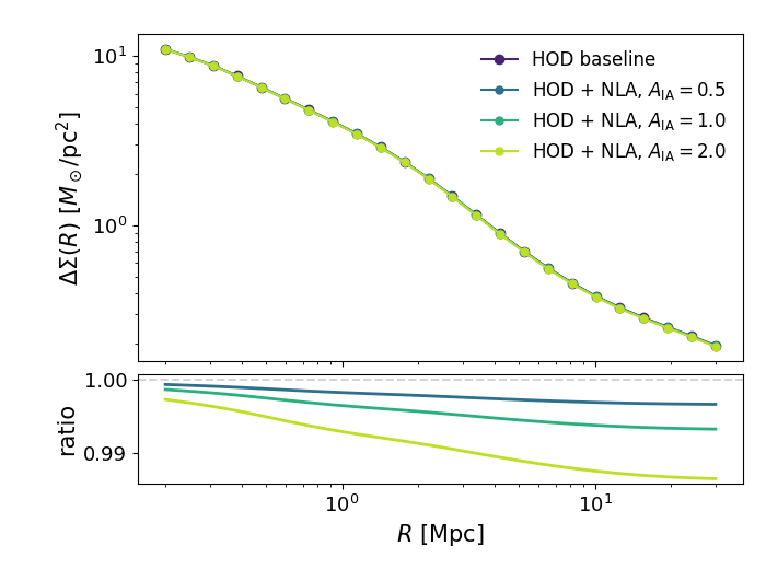
The NLA contribution can be varied through the intrinsic-alignment amplitude
A_IA. This example compares a baseline HOD model with three NLA strengths
while keeping the same projected-radius grid and lens redshift.
import cmasher as cmr
import matplotlib.pyplot as plt
import numpy as np

from dsf.data_vector.delta_sigma_builder import DeltaSigmaCalculator
from dsf.modelling import (
    make_ccl_cosmology,
    pk2d_hod,
    pk2d_hod_with_nla,
)


cosmo = make_ccl_cosmology(
    transfer_function="eisenstein_hu",
    matter_power_spectrum="halofit",
)

r = np.geomspace(0.2, 30.0, 24)
z_lens = 0.55
a_lens = 1.0 / (1.0 + z_lens)

k_array = np.geomspace(1.0e-3, 30.0, 64)
a_array = np.linspace(0.3, 1.0, 16)


def pk2d_baseline(*, cosmo):
    return pk2d_hod(
        cosmo,
        k_array=k_array,
        a_array=a_array,
    )


baseline_calculator = DeltaSigmaCalculator(pk2d_func=pk2d_baseline)

delta_sigma_baseline = baseline_calculator.delta_sigma(
    r=r,
    a=a_lens,
    cosmo=cosmo,
)

ia_amplitudes = [0.5, 1.0, 2.0]

colors = cmr.take_cmap_colors(
    "viridis",
    len(ia_amplitudes) + 1,
    cmap_range=(0.10, 0.90),
    return_fmt="hex",
)

fig, (ax, ax_res) = plt.subplots(
    2,
    1,
    figsize=(7.0, 5.2),
    sharex=True,
    gridspec_kw={"height_ratios": [3.0, 1.0], "hspace": 0.06},
)

ax.plot(
    r,
    delta_sigma_baseline,
    color=colors[0],
    marker="o",
    markersize=6,
    label="HOD baseline",
)

for color, A_IA in zip(colors[1:], ia_amplitudes):

    def pk2d_func(*, cosmo, A_IA=A_IA):
        return pk2d_hod_with_nla(
            cosmo,
            k_array=k_array,
            a_array=a_array,
            A_IA=A_IA,
            a_bias=a_lens,
        )

    calculator = DeltaSigmaCalculator(pk2d_func=pk2d_func)

    delta_sigma_ia = calculator.delta_sigma(
        r=r,
        a=a_lens,
        cosmo=cosmo,
    )

    ax.plot(
        r,
        delta_sigma_ia,
        color=color,
        marker="o",
        markersize=5,
        label=rf"HOD + NLA, $A_{{\rm IA}}={A_IA:.1f}$",
    )

    ax_res.plot(
        r,
        delta_sigma_ia / delta_sigma_baseline,
        color=color,
        linewidth=2.0,
    )

ax.set_xscale("log")
ax.set_yscale("log")
ax.set_ylabel(r"$\Delta\Sigma(R)\ [M_\odot / {\rm pc}^2]$", fontsize=15)
ax.tick_params(axis="both", which="major", labelsize=13)
ax.tick_params(axis="both", which="minor", labelsize=11)
ax.legend(fontsize=12, frameon=False)

ax_res.axhline(1.0, color="lightgray", linewidth=1.4, linestyle="--")
ax_res.set_xscale("log")
ax_res.set_ylabel("ratio", fontsize=15)
ax_res.set_xlabel(r"$R\ [{\rm Mpc}]$", fontsize=15)
ax_res.tick_params(axis="both", which="major", labelsize=13)
ax_res.tick_params(axis="both", which="minor", labelsize=11)

fig.subplots_adjust(left=0.18, right=0.97, bottom=0.15, top=0.94)

plt.show()
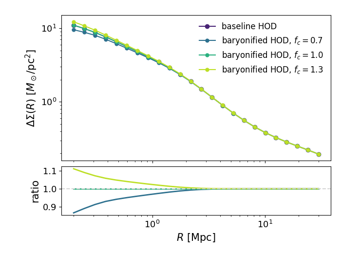
Baryonification strength variants
The baryonified HOD model rescales the halo concentration relation through the
parameter f_c. Values below unity suppress concentrations relative to the
baseline Duffy relation, while values above unity increase concentrations.
import cmasher as cmr
import matplotlib.pyplot as plt
import numpy as np

from dsf.data_vector.delta_sigma_builder import DeltaSigmaCalculator
from dsf.modelling import (
    make_ccl_cosmology,
    pk2d_hod,
    pk2d_hod_baryonified,
)


cosmo = make_ccl_cosmology(
    transfer_function="eisenstein_hu",
    matter_power_spectrum="halofit",
)

r = np.geomspace(0.2, 30.0, 24)

z_lens = 0.55
a_lens = 1.0 / (1.0 + z_lens)

k_array = np.geomspace(1.0e-3, 30.0, 64)
a_array = np.linspace(0.3, 1.0, 16)


def pk2d_baseline(*, cosmo):
    return pk2d_hod(
        cosmo,
        k_array=k_array,
        a_array=a_array,
    )


baseline_calculator = DeltaSigmaCalculator(
    pk2d_func=pk2d_baseline,
)

delta_sigma_baseline = baseline_calculator.delta_sigma(
    r=r,
    a=a_lens,
    cosmo=cosmo,
)

baryon_levels = [0.7, 1.0, 1.3]

colors = cmr.take_cmap_colors(
    "viridis",
    len(baryon_levels) + 1,
    cmap_range=(0.10, 0.90),
    return_fmt="hex",
)

fig, (ax, ax_res) = plt.subplots(
    2,
    1,
    figsize=(7.0, 5.2),
    sharex=True,
    gridspec_kw={"height_ratios": [3.0, 1.0], "hspace": 0.06},
)

ax.plot(
    r,
    delta_sigma_baseline,
    color=colors[0],
    marker="o",
    markersize=6,
    label="baseline HOD",
)

for color, f_c in zip(colors[1:], baryon_levels):

    def pk2d_func(*, cosmo, f_c=f_c):
        return pk2d_hod_baryonified(
            cosmo,
            k_array=k_array,
            a_array=a_array,
            f_c=f_c,
        )

    calculator = DeltaSigmaCalculator(pk2d_func=pk2d_func)

    delta_sigma_baryons = calculator.delta_sigma(
        r=r,
        a=a_lens,
        cosmo=cosmo,
    )

    ax.plot(
        r,
        delta_sigma_baryons,
        color=color,
        marker="o",
        markersize=5,
        label=rf"baryonified HOD, $f_c={f_c:.1f}$",
    )

    ax_res.plot(
        r,
        delta_sigma_baryons / delta_sigma_baseline,
        color=color,
        linewidth=2.0,
    )

ax.set_xscale("log")
ax.set_yscale("log")

ax.set_ylabel(
    r"$\Delta\Sigma(R)\ [M_\odot / {\rm pc}^2]$",
    fontsize=15,
)

ax.tick_params(axis="both", which="major", labelsize=13)
ax.tick_params(axis="both", which="minor", labelsize=11)

ax.legend(
    fontsize=12,
    frameon=False,
)

ax_res.axhline(
    1.0,
    color="lightgray",
    linewidth=1.4,
    linestyle="--",
)

ax_res.plot([], [])

ax_res.set_xscale("log")
ax_res.set_ylabel("ratio", fontsize=15)
ax_res.set_xlabel(r"$R\ [{\rm Mpc}]$", fontsize=15)

ax_res.tick_params(axis="both", which="major", labelsize=13)
ax_res.tick_params(axis="both", which="minor", labelsize=11)

fig.subplots_adjust(
    left=0.18,
    right=0.97,
    bottom=0.15,
    top=0.94,
)

plt.show()
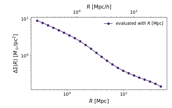
Using projected radius in Mpc and Mpc / h
Some forecast inputs and observational data vectors are tabulated in
Mpc / h. In this case, convert the radius grid before passing it to
DeltaSigmaCalculator if the calculator expects radii in Mpc. The plot
below shows both conventions with a secondary x-axis.
import cmasher as cmr
import matplotlib.pyplot as plt
import numpy as np

from dsf.data_vector.delta_sigma_builder import DeltaSigmaCalculator
from dsf.modelling import make_ccl_cosmology, pk2d_hod


cosmo = make_ccl_cosmology(
    transfer_function="eisenstein_hu",
    matter_power_spectrum="halofit",
)

h = cosmo["h"]

r_mpc_over_h = np.geomspace(0.2, 30.0, 24)
r_mpc = r_mpc_over_h / h

z_lens = 0.55
a_lens = 1.0 / (1.0 + z_lens)

k_array = np.geomspace(1.0e-3, 30.0, 64)
a_array = np.linspace(0.3, 1.0, 16)


def pk2d_func(*, cosmo):
    return pk2d_hod(
        cosmo,
        k_array=k_array,
        a_array=a_array,
    )


calculator = DeltaSigmaCalculator(pk2d_func=pk2d_func)

delta_sigma = calculator.delta_sigma(
    r=r_mpc,
    a=a_lens,
    cosmo=cosmo,
)

colors = cmr.take_cmap_colors(
    "viridis",
    2,
    cmap_range=(0.10, 0.90),
    return_fmt="hex",
)

fig, ax = plt.subplots(figsize=(7.0, 4.4))

ax.plot(
    r_mpc,
    delta_sigma,
    color=colors[0],
    marker="o",
    markersize=6,
    label=r"evaluated with $R\ [{\rm Mpc}]$",
)

ax.set_xscale("log")
ax.set_yscale("log")
ax.set_xlabel(r"$R\ [{\rm Mpc}]$", fontsize=15)
ax.set_ylabel(r"$\Delta\Sigma(R)\ [M_\odot / {\rm pc}^2]$", fontsize=15)
ax.tick_params(axis="both", which="major", labelsize=13)
ax.tick_params(axis="both", which="minor", labelsize=11)
ax.legend(fontsize=12, frameon=False)

ax_top = ax.secondary_xaxis(
    "top",
    functions=(
        lambda r_mpc: r_mpc * h,
        lambda r_mpc_over_h: r_mpc_over_h / h,
    ),
)

ax_top.set_xscale("log")
ax_top.set_xlabel(r"$R\ [{\rm Mpc}/h]$", fontsize=15)
ax_top.tick_params(axis="x", which="major", labelsize=13)
ax_top.tick_params(axis="x", which="minor", labelsize=11)

fig.subplots_adjust(left=0.18, right=0.97, bottom=0.17, top=0.84)

plt.show()
Notes
The single-redshift calculation evaluates
at one lens scale factor. The lens-bin-averaged calculation instead integrates the signal over a toy lens redshift distribution,
The lower panel shows the ratio between the lens-bin-averaged signal and the single-redshift signal. This is useful for checking how much redshift averaging changes the projected signal relative to evaluating the model at one effective lens redshift.
The model-variant examples use the same DeltaSigmaCalculator interface but
swap the Pk2D model supplied through pk2d_func. This keeps the data-vector
evaluation fixed while changing the physical ingredients entering the
galaxy-matter power spectrum. The NLA examples show how intrinsic-alignment
strength changes the signal through A_IA. The baryonified examples show how a
modified concentration relation can propagate into the projected
\(\Delta\Sigma\) prediction.
All data-vector outputs are arrays with the same length as the input projected radius grid.
Unit convention
The calculator examples above pass projected radii in Mpc. If a data vector
or forecast configuration is instead tabulated in Mpc / h, convert the grid
before evaluating the signal,
The Mpc / h example does this conversion explicitly, but plots the result
against the original Mpc / h grid. This makes the convention visible without
silently changing the units expected by DeltaSigmaCalculator.
Before comparing DSF outputs to external measurements, make sure the radius
grid, mass convention, surface-density convention, and any powers of h are
handled consistently.