DeltaSigma covariance

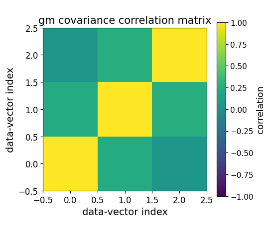
This example shows how to compute a minimal DSF covariance matrix for the current \(\Delta\Sigma(R)\) forecast data vector.

At present, the forecast builder uses the gm block-diagonal covariance, because the forecast data vector is \(\Delta\Sigma\)-only. In other words, the covariance used by the current forecast workflow is the gm x gm block.

The documentation examples are runnable, so this example intentionally uses a small redshift grid, a small number of bins, one lens-source pair, a short radius grid, and a lightweight Hankel setup. For a real analysis, these settings should be made more accurate, and covariance evaluation will naturally take longer.

Minimal gm covariance example

import matplotlib.pyplot as plt
import numpy as np

from dsf.covariance.cov_builder import DeltaSigmaCovarianceBuilder
from dsf.modelling import make_ccl_cosmology
from dsf.tomography.tomo_builder import TomographyBuilder


cosmo = make_ccl_cosmology(
    transfer_function="eisenstein_hu",
    matter_power_spectrum="halofit",
)

z = np.linspace(0.05, 1.8, 80)

tomography = TomographyBuilder(
    lens_survey="lsst",
    source_survey="lsst",
    lens_sample=None,
    source_sample=None,
    lens_year="1",
    source_year="1",
    lens_role="lens",
    source_role="source",
    overlap_threshold=0.10,
    source_behind_lens=True,
    shared_overrides={
        "bins": {
            "count": 2,
        },
    },
)

tomo_inputs = tomography.prepare_bins()

bin_pairs = tomo_inputs["bin_pairs"][:1]
rp_bin_edges = np.geomspace(2.0, 20.0, 4)

covariance_builder = DeltaSigmaCovarianceBuilder(
    cosmo=cosmo,
    lens_result=tomo_inputs["lens_result"],
    source_result=tomo_inputs["source_result"],
    lens_population_stats=tomo_inputs["lens_population_stats"],
    source_population_stats=tomo_inputs["source_population_stats"],
    bin_pairs=bin_pairs,
    rp_bin_edges=rp_bin_edges,
    area_deg2=5000.0,
    sigma_e=0.26,
    galaxy_bias=1.5,
    k=np.geomspace(2.0e-2, 5.0, 48),
    hankel_kwargs={
        "r_min": 1.5,
        "r_max": 25.0,
        "k_min": 2.0e-2,
        "k_max": 5.0,
        "orders": (2,),
        "n_zeros": 250,
        "n_zeros_step": 100,
        "prune_r": 4,
        "verbose": False,
        "max_iterations": 20,
    },
    taper=False,
)

pairs, cov_gm = covariance_builder.gm_block_diagonal()
errors = covariance_builder.diagonal_error(cov_gm)
corr = covariance_builder.correlation_matrix(cov_gm)

print("Selected bin pairs:", pairs)
print("gm covariance shape:", cov_gm.shape)
print("diagonal error shape:", errors.shape)
print("diagonal errors:", errors)

fig, ax = plt.subplots(figsize=(5.4, 4.6))

image = ax.imshow(
    corr,
    vmin=-1.0,
    vmax=1.0,
    origin="lower",
)

ax.set_title("gm covariance correlation matrix", fontsize=15)
ax.set_xlabel("data-vector index", fontsize=14)
ax.set_ylabel("data-vector index", fontsize=14)
ax.tick_params(axis="both", which="major", labelsize=12)

cbar = fig.colorbar(image, ax=ax)
cbar.set_label("correlation", fontsize=13)
cbar.ax.tick_params(labelsize=11)

fig.subplots_adjust(left=0.16, right=0.92, bottom=0.14, top=0.90)

plt.show()

Notes

The call

pairs, cov_gm = covariance_builder.gm_block_diagonal()

returns a block-diagonal covariance matrix assembled from the gm x gm covariance block for each selected lens-source bin pair.

The returned covariance has shape

\[(N_{\rm pair} N_R, N_{\rm pair} N_R),\]

where \(N_{\rm pair}\) is the number of selected lens-source bin pairs and \(N_R\) is the number of projected-radius bins.

Diagonal errors can be extracted with

errors = covariance_builder.diagonal_error(cov_gm)

These are the one-sigma errors from the square root of the covariance diagonal.