End-to-end forecast
This example demonstrates an end-to-end \(\Delta\Sigma(R)\) Fisher forecast workflow with DSF.
The workflow combines:
tomographic lens/source bin construction,
fiducial \(\Delta\Sigma\) data-vector generation,
matched
gmcovariance construction,Fisher-matrix evaluation with
ForecastKit,Gaussian priors,
and GetDist posterior visualization.
The compact interface passed to the forecast tool is
model, theta0, cov = builder.forecast_inputs()
Here, model maps a parameter vector to the stacked
\(\Delta\Sigma\) data vector, theta0 stores the fiducial HOD
parameters, and cov is the matched covariance matrix.
This example varies two HOD parameters, log10Mmin_0 and log10M1_0,
through the supplied pk2d_func.
Because covariance construction is the most expensive step, the example caches the computed forecast products and Fisher matrices. If the cache file exists, the plot is rebuilt from the cached arrays. If the cache file is missing, the forecast is recomputed and the cache is written.
Forecast-builder example
from pathlib import Path

import cmasher as cmr
import numpy as np

from derivkit import ForecastKit
from getdist import plots as getdist_plots

from dsf.delta_sigma_forecast_builder import DeltaSigmaForecastBuilder
from dsf.modelling import make_ccl_cosmology, pk2d_hod


np.set_printoptions(precision=8, suppress=True)

cache_path = Path("cached_files/builder_example_forecast_cache.npz")

parameter_names = ["log10Mmin_0", "log10M1_0"]
parameter_labels = [
    r"\log_{10}(M_{\min}/[h^{-1}M_\odot])",
    r"\log_{10}(M_1/[h^{-1}M_\odot])",
]
sigma_prior = np.array([0.50, 0.70], dtype=float)
fisher_prior = np.diag(1.0 / sigma_prior**2)

if cache_path.exists():
    cached = np.load(cache_path)

    theta0 = cached["theta0"]
    r = cached["r"]
    data_vector = cached["data_vector"]
    cov = cached["cov"]
    fisher_like = cached["fisher_like"]
    fisher_post = cached["fisher_post"]
    bin_pairs = [tuple(pair) for pair in cached["bin_pairs"]]

else:
    cache_path.parent.mkdir(parents=True, exist_ok=True)

    cosmo = make_ccl_cosmology(
        transfer_function="eisenstein_hu",
        matter_power_spectrum="halofit",
    )

    theta0 = np.array([12.5, 13.5])

    r = np.geomspace(2.0, 25.0, 5)
    rp_bin_edges = np.geomspace(2.0, 25.0, 6)

    k_array = np.geomspace(1.0e-3, 20.0, 40)
    a_array = np.linspace(0.35, 1.0, 10)


    def pk2d_func(*, cosmo, log10Mmin_0=12.5, log10M1_0=13.5):
        return pk2d_hod(
            cosmo,
            k_array=k_array,
            a_array=a_array,
            log10Mmin_0=log10Mmin_0,
            log10M1_0=log10M1_0,
        )


    def theta_mapper(theta, context):
        log10Mmin_0, log10M1_0 = theta

        return {
            "cosmo": context["cosmo"],
            "pk2d_kwargs": {
                "log10Mmin_0": float(log10Mmin_0),
                "log10M1_0": float(log10M1_0),
            },
        }


    builder = DeltaSigmaForecastBuilder(
        cosmo=cosmo,
        pk2d_func=pk2d_func,
        theta0=theta0,
        parameter_names=parameter_names,
        theta_mapper=theta_mapper,
        r=r,
        rp_bin_edges=rp_bin_edges,
        area_deg2=1000.0,
        sigma_e=0.26,
        lens_survey="lsst",
        source_survey="lsst",
        lens_sample=None,
        source_sample=None,
        lens_year="1",
        source_year="1",
        lens_role="lens",
        source_role="source",
        overlap_threshold=1.0,
        source_behind_lens=True,
        shared_overrides={
            "bins": {
                "n_bins": 2,
            },
        },
        galaxy_bias=1.5,
        k=np.geomspace(1.0e-2, 10.0, 40),
        hankel_kwargs={
            "r_min": 1.0,
            "r_max": 35.0,
            "k_min": 1.0e-2,
            "k_max": 10.0,
            "orders": (2,),
            "n_zeros": 250,
            "n_zeros_step": 100,
            "prune_r": 4,
            "verbose": False,
            "max_iterations": 30,
        },
        taper=False,
        verbose=False,
    )

    forecast = builder.prepare()

    model, theta0, cov = builder.forecast_inputs()
    data_vector = forecast["fiducial_data_vector"]
    bin_pairs = forecast["bin_pairs"]

    jitter = 1.0e-8 * np.max(np.diag(cov))
    cov = cov + jitter * np.eye(cov.shape[0])

    fk = ForecastKit(
        function=model,
        theta0=theta0,
        cov=cov,
    )

    fisher_like = fk.fisher(
        method="finite",
        stepsize=1.0e-2,
        num_points=3,
    )

    fisher_post = fisher_like + fisher_prior

    np.savez(
        cache_path,
        theta0=theta0,
        r=r,
        data_vector=data_vector,
        cov=cov,
        fisher_like=fisher_like,
        fisher_post=fisher_post,
        bin_pairs=np.asarray(bin_pairs, dtype=int),
    )

print("Selected bin pairs:", bin_pairs)
print("Fiducial theta0:", theta0)
print("Fiducial data-vector shape:", data_vector.shape)
print("Covariance shape:", cov.shape)

print("Likelihood-only Fisher matrix:")
print(fisher_like)

print("Prior Fisher matrix:")
print(fisher_prior)

print("Posterior Fisher matrix:")
print(fisher_post)

print("Likelihood-only parameter sigma:")
print(np.sqrt(np.diag(np.linalg.inv(fisher_like))))

print("Posterior parameter sigma:")
print(np.sqrt(np.diag(np.linalg.inv(fisher_post))))

fk_plot = ForecastKit(
    function=lambda theta: np.asarray(theta, dtype=float),
    theta0=theta0,
    cov=np.eye(len(theta0)),
)

g_like = fk_plot.getdist_fisher_gaussian(
    fisher=fisher_like,
    names=parameter_names,
    labels=parameter_labels,
    label="Fisher",
)

g_post = fk_plot.getdist_fisher_gaussian(
    fisher=fisher_post,
    names=parameter_names,
    labels=parameter_labels,
    label="Fisher + Gaussian prior",
)

colors = cmr.take_cmap_colors(
    "viridis",
    2,
    cmap_range=(0.10, 0.90),
    return_fmt="hex",
)

line_width = 1.5

plotter = getdist_plots.get_subplot_plotter(width_inch=4.5)
plotter.settings.linewidth_contour = line_width
plotter.settings.linewidth = line_width
plotter.settings.figure_legend_frame = False
plotter.settings.legend_rect_border = False

plotter.triangle_plot(
    [g_like, g_post],
    params=parameter_names,
    filled=[False, False],
    contour_colors=[colors[0], colors[1]],
    contour_lws=[line_width, line_width],
    contour_ls=["-", "-"],
)

(g_like is not None) and (g_post is not None)
Fisher input interface
The compact forecast interface is
model, theta0, cov = builder.forecast_inputs()
The returned model is a callable that maps a parameter vector to the stacked
\(\Delta\Sigma\) data vector. The returned theta0 is the fiducial
parameter vector, and cov is the matched gm covariance matrix.
In this example, the forecast parameters enter through the HOD power-spectrum model,
This makes the example useful as an end-to-end test of the forecast plumbing before moving to richer SHMR, baryonic, intrinsic-alignment, or cosmological parameterizations.
Gaussian priors
The Fisher matrix computed from the forecast data vector represents the likelihood-only information. A Gaussian prior can be added directly at the Fisher-matrix level,
where, for independent Gaussian priors,
The example above uses
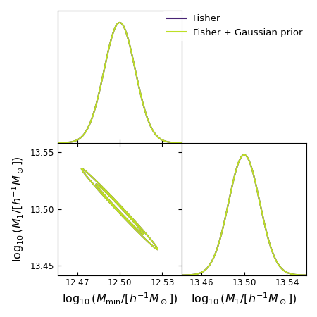
The plotted contours compare the likelihood-only Fisher result with the posterior Fisher result after adding these Gaussian priors.
Caching
The first execution builds the forecast products and writes
docs/examples/builder_example_forecast_cache.npz
Subsequent documentation builds load the cached arrays and only recreate the GetDist Gaussian objects and plot. This keeps the example reproducible while avoiding repeated covariance construction during normal documentation builds.
Notes
This is a toy example intended to demonstrate the DSF forecast workflow and software interface. It is not meant to represent a production LSST DESC forecast analysis. Production forecast configurations, analysis scripts, and survey-specific choices live in the companion analysis repository: LSSTDESC/dsf-analysis.
DeltaSigmaForecastBuilder builds and caches the forecast products. Calling
forecast = builder.prepare()
returns a dictionary with the fiducial data vector, selected bin pairs, tomography products, covariance builder, and shared forecast context.
Calling
model, theta0, cov = builder.forecast_inputs()
returns only the minimal forecast inputs. This is the interface expected by many Fisher or DALI workflows.
Extending the same workflow to DALI is also straightforward through
ForecastKit. For an example of sampling a DALI posterior with emcee,
see the
DerivKit DALI example.
The current builder uses the gm block-diagonal covariance because the
forecast data vector is \(\Delta\Sigma\)-only. Future joint builders can add
matched data vectors for additional covariance blocks.