Example 1: Ideal data
Fit halo mass to shear profile with ideal data
the LSST-DESC CLMM team
This notebook demonstrates how to use clmm to estimate a WL halo
mass of a galaxy cluster in the ideal case: i) all galaxies on a single
source plane, ii) no redshift errors, iii) no shape noise. The steps
below correspond to: - Setting things up, with the proper imports. -
Generating a ideal mock dataset. - Computing the binned reduced
tangential shear profile, for two different binning scheme. - Setting up
the model to be fitted to the data. - Perform a simple fit using
scipy.optimize.basinhopping and visualize the results.
Setup
First, we import some standard packages.
import numpy as np
import matplotlib.pyplot as plt

from numpy import random
Next, we import clmm’s core modules.
import clmm
import clmm.dataops as da
import clmm.galaxycluster as gc
import clmm.theory as theory
from clmm import Cosmology
Make sure we know which version we’re using
clmm.__version__
'1.12.0'
We then import a support modules for a specific data sets. clmm
includes support modules that enable the user to generate mock data in a
format compatible with clmm. We also provide support modules for
processing other specific data sets for use with clmm. Any existing
support module can be used as a template for creating a new support
module for another data set. If you do make such a support module,
please do consider making a pull request so we can add it for others to
use.
Making mock data
from clmm.support import mock_data as mock
np.random.seed(11)
To create mock data, we need to define a true cosmology.
mock_cosmo = Cosmology(H0=70.0, Omega_dm0=0.27 - 0.045, Omega_b0=0.045, Omega_k0=0.0)
We now set some parameters for a mock galaxy cluster.
cosmo = mock_cosmo
cluster_id = "Awesome_cluster"
cluster_m = 1.0e15  # M200,m [Msun]
cluster_z = 0.3
src_z = 0.8
concentration = 4
ngals = 10000
cluster_ra = 20.0
cluster_dec = 30.0
Then we use the mock_data support module to generate a new galaxy
catalog.
ideal_data = mock.generate_galaxy_catalog(
    cluster_m,
    cluster_z,
    concentration,
    cosmo,
    src_z,
    ngals=ngals,
    cluster_ra=cluster_ra,
    cluster_dec=cluster_dec,
)
This galaxy catalog is then converted to a clmm.GalaxyCluster
object.
gc_object = clmm.GalaxyCluster(cluster_id, cluster_ra, cluster_dec, cluster_z, ideal_data)
A clmm.GalaxyCluster object can be pickled and saved for later use.
gc_object.save("mock_GC.pkl")
Any saved clmm.GalaxyCluster object may be read in for analysis.
cl = clmm.GalaxyCluster.load("mock_GC.pkl")
print("Cluster info = ID:", cl.unique_id, "; ra:", cl.ra, "; dec:", cl.dec, "; z_l :", cl.z)
print("The number of source galaxies is :", len(cl.galcat))

ra_l = cl.ra
dec_l = cl.dec
z = cl.z
e1 = cl.galcat["e1"]
e2 = cl.galcat["e2"]
ra_s = cl.galcat["ra"]
dec_s = cl.galcat["dec"]
z_s = cl.galcat["z"]
Cluster info = ID: Awesome_cluster ; ra: 20.0 ; dec: 30.0 ; z_l : 0.3
The number of source galaxies is : 10000
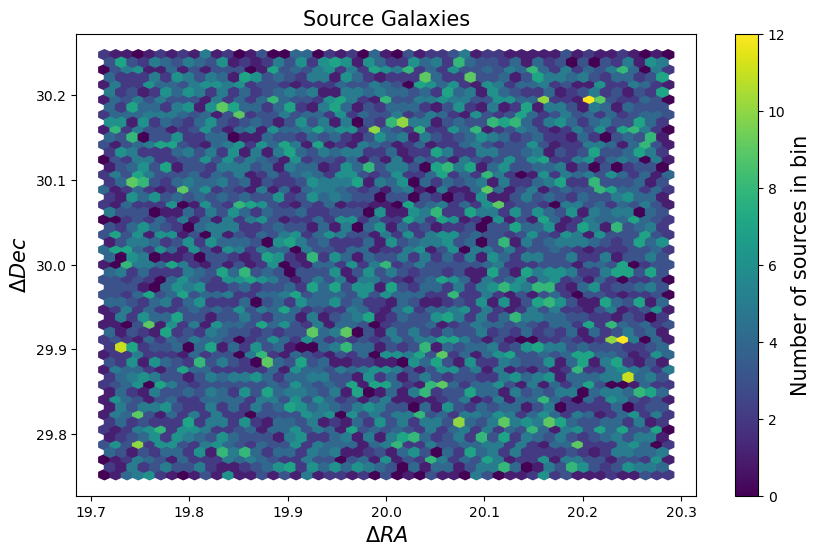
We can visualize the distribution of galaxies on the sky.
fsize = 15

fig = plt.figure(figsize=(10, 6))
hb = fig.gca().hexbin(ra_s, dec_s, gridsize=50)

cb = fig.colorbar(hb)
cb.set_label("Number of sources in bin", fontsize=fsize)

plt.gca().set_xlabel(r"$\Delta RA$", fontsize=fsize)
plt.gca().set_ylabel(r"$\Delta Dec$", fontsize=fsize)
plt.gca().set_title("Source Galaxies", fontsize=fsize)

plt.show()
clmm separates cosmology-dependent and cosmology-independent
functionality.
Deriving observables
We first demonstrate a few of the procedures one can perform on data without assuming a cosmology.
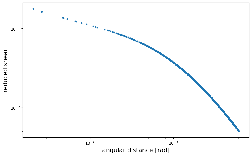
Computing shear
clmm.dataops.compute_tangential_and_cross_components calculates the
tangential and cross shears for each source galaxy in the cluster.
theta, g_t, g_x = da.compute_tangential_and_cross_components(ra_l, dec_l, ra_s, dec_s, e1, e2)
We can visualize the shear field at each galaxy location.
fig = plt.figure(figsize=(10, 6))

fig.gca().loglog(theta, g_t, ".")
plt.ylabel("reduced shear", fontsize=fsize)
plt.xlabel("angular distance [rad]", fontsize=fsize)
Text(0.5, 0, 'angular distance [rad]')
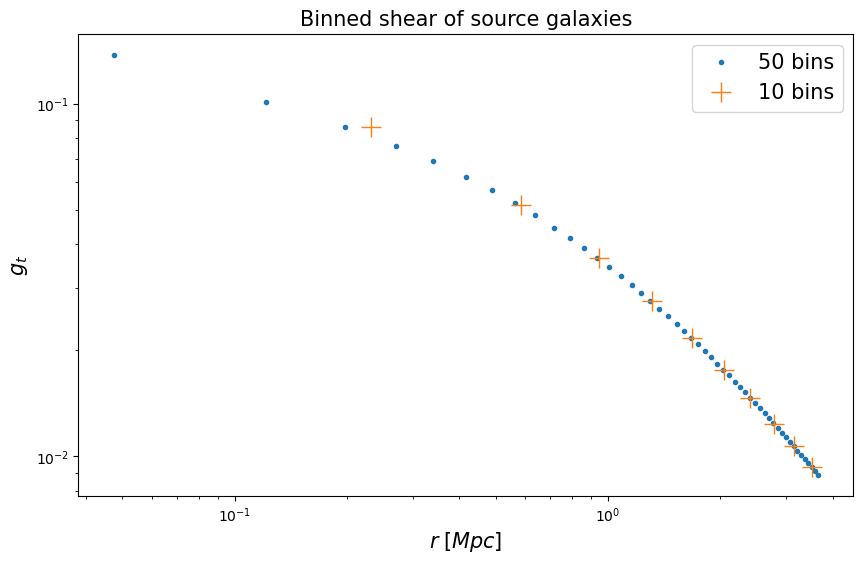
Radially binning the data
Here we compare the reconstructed mass under two different bin definitions.
Note binning would cause fitted mass to be slightly larger than input mass. The reason is that g(r), the tangential reduced shear along cluster radius, is a convex function – the function value after binning would be larger, but the bias becomes smaller as bin number increases.
bin_edges1 = da.make_bins(0.01, 3.7, 50)
bin_edges2 = da.make_bins(0.01, 3.7, 10)
clmm.dataops.make_radial_profile evaluates the average shear of the
galaxy catalog in bins of radius.
res1 = da.make_radial_profile(
    [g_t, g_x, z_s],
    theta,
    "radians",
    "Mpc",
    bins=bin_edges1,
    cosmo=cosmo,
    z_lens=z,
    include_empty_bins=False,
)
res2 = da.make_radial_profile(
    [g_t, g_x, z_s],
    theta,
    "radians",
    "Mpc",
    bins=bin_edges2,
    cosmo=cosmo,
    z_lens=z,
    include_empty_bins=False,
)
/global/homes/a/aguena/.local/perlmutter/python-3.11/lib/python3.11/site-packages/clmm-1.12.0-py3.11.egg/clmm/utils/statistic.py:97: RuntimeWarning: invalid value encountered in sqrt
/global/homes/a/aguena/.local/perlmutter/python-3.11/lib/python3.11/site-packages/clmm-1.12.0-py3.11.egg/clmm/utils/statistic.py:97: RuntimeWarning: invalid value encountered in sqrt
Note that we set include_empty_bins=False explicitly here even
though it is the default behavior. Setting the argument to True
would also return empty bins (that is, bins with at most one data
point in them), which would have to be excluded manually when fitting,
though it might be useful e.g., when combining datasets. To clarify the
behavior, consider the following comparison:
res_with_empty = da.make_radial_profile(
    [g_t, g_x, z_s],
    theta,
    "radians",
    "Mpc",
    bins=1000,
    cosmo=cosmo,
    z_lens=z,
    include_empty_bins=True,
)
# this is the default behavior
res_without_empty = da.make_radial_profile(
    [g_t, g_x, z_s],
    theta,
    "radians",
    "Mpc",
    bins=1000,
    cosmo=cosmo,
    z_lens=z,
    include_empty_bins=False,
)
res_with_empty["n_src"].size, res_without_empty["n_src"].size
/global/homes/a/aguena/.local/perlmutter/python-3.11/lib/python3.11/site-packages/clmm-1.12.0-py3.11.egg/clmm/utils/statistic.py:97: RuntimeWarning: invalid value encountered in sqrt
/global/homes/a/aguena/.local/perlmutter/python-3.11/lib/python3.11/site-packages/clmm-1.12.0-py3.11.egg/clmm/utils/statistic.py:97: RuntimeWarning: invalid value encountered in sqrt
/global/homes/a/aguena/.local/perlmutter/python-3.11/lib/python3.11/site-packages/clmm-1.12.0-py3.11.egg/clmm/utils/statistic.py:97: RuntimeWarning: invalid value encountered in sqrt
/global/homes/a/aguena/.local/perlmutter/python-3.11/lib/python3.11/site-packages/clmm-1.12.0-py3.11.egg/clmm/utils/statistic.py:97: RuntimeWarning: invalid value encountered in sqrt
(1000, 892)
i.e., 108 bins have fewer than two sources in them and are excluded by default (when setting the random seed to 11).
For later use, we’ll define some variables for the binned radius and tangential shear.
gt_profile1 = res1["p_0"]
r1 = res1["radius"]
z1 = res1["p_2"]

gt_profile2 = res2["p_0"]
r2 = res2["radius"]
z2 = res2["p_2"]
We visualize the radially binned shear for our mock galaxies.
fig = plt.figure(figsize=(10, 6))

fig.gca().loglog(r1, gt_profile1, ".", label="50 bins")
fig.gca().loglog(r2, gt_profile2, "+", markersize=15, label="10 bins")
plt.legend(fontsize=fsize)

plt.gca().set_title(r"Binned shear of source galaxies", fontsize=fsize)
plt.gca().set_xlabel(r"$r\;[Mpc]$", fontsize=fsize)
plt.gca().set_ylabel(r"$g_t$", fontsize=fsize)
Text(0, 0.5, '$g_t$')
You can also run make_radial_profile direct on a
clmm.GalaxyCluster object.
cl.compute_tangential_and_cross_components()  # You need to add the shear components first
cl.make_radial_profile("Mpc", bins=1000, cosmo=cosmo, include_empty_bins=False)
pass
/global/homes/a/aguena/.local/perlmutter/python-3.11/lib/python3.11/site-packages/clmm-1.12.0-py3.11.egg/clmm/utils/statistic.py:97: RuntimeWarning: invalid value encountered in sqrt
/global/homes/a/aguena/.local/perlmutter/python-3.11/lib/python3.11/site-packages/clmm-1.12.0-py3.11.egg/clmm/utils/statistic.py:97: RuntimeWarning: invalid value encountered in sqrt
After running clmm.GalaxyCluster.make_radial_profile object, the
object acquires the clmm.GalaxyCluster.profile attribute.
for n in cl.profile.colnames:
    cl.profile[n].format = "%6.3e"
cl.profile.pprint(max_width=-1)
radius_min   radius  radius_max     gt      gt_err      gx       gx_err      z       z_err     n_src      W_l
---------- --------- ---------- --------- --------- ---------- --------- --------- --------- --------- ---------
 1.929e-02 2.182e-02  2.490e-02 1.699e-01 4.854e-03 -8.478e-17 1.073e-18 8.000e-01 0.000e+00 2.000e+00 2.000e+00
 4.172e-02 4.415e-02  4.733e-02 1.354e-01 7.376e-05 -6.592e-17 2.453e-18 8.000e-01 0.000e+00 2.000e+00 2.000e+00
 5.855e-02 6.252e-02  6.416e-02 1.224e-01 2.610e-04 -5.898e-17 2.453e-18 8.000e-01 0.000e+00 2.000e+00 2.000e+00
 1.595e-01 1.611e-01  1.651e-01 9.224e-02 7.363e-05 -4.163e-17 4.907e-18 8.000e-01 0.000e+00 2.000e+00 2.000e+00
 1.931e-01 1.937e-01  1.987e-01 8.657e-02 3.080e-05 -3.990e-17 1.227e-18 8.000e-01 0.000e+00 2.000e+00 2.000e+00
 2.100e-01 2.141e-01  2.156e-01 8.349e-02 9.282e-05 -1.735e-17 1.227e-17 8.000e-01 0.000e+00 2.000e+00 2.000e+00
 2.156e-01 2.186e-01  2.212e-01 8.283e-02 1.114e-04 -4.077e-17 4.089e-19 8.000e-01 0.000e+00 3.000e+00 3.000e+00
 2.324e-01 2.357e-01  2.380e-01 8.049e-02 8.085e-05 -1.973e-17 1.395e-17 8.000e-01 0.000e+00 2.000e+00 2.000e+00
 2.604e-01 2.644e-01  2.660e-01 7.687e-02 1.141e-05 -2.017e-17 1.181e-17 8.000e-01 0.000e+00 2.000e+00 2.000e+00
 2.773e-01 2.800e-01  2.829e-01 7.505e-02 4.587e-05 -1.041e-17 9.342e-18 8.000e-01 0.000e+00 4.000e+00 4.000e+00
 2.885e-01 2.898e-01  2.941e-01 7.396e-02 4.115e-05 -3.426e-17 3.756e-19 8.000e-01 0.000e+00 4.000e+00 4.000e+00
 3.053e-01 3.084e-01  3.109e-01 7.197e-02 9.003e-05 -2.125e-17 1.012e-17 8.000e-01 0.000e+00 2.000e+00 2.000e+00
 3.109e-01 3.134e-01  3.165e-01 7.146e-02 2.563e-05 -2.353e-17 8.827e-18 8.000e-01 0.000e+00 4.000e+00 4.000e+00
 3.389e-01 3.407e-01  3.446e-01 6.877e-02 8.012e-05 -3.441e-17 2.361e-19 8.000e-01 0.000e+00 3.000e+00 3.000e+00
 3.614e-01 3.642e-01  3.670e-01 6.661e-02 9.981e-05 -3.383e-17 6.133e-19 8.000e-01 0.000e+00 2.000e+00 2.000e+00
 3.726e-01 3.750e-01  3.782e-01 6.567e-02 1.123e-06 -3.469e-17 4.907e-18 8.000e-01 0.000e+00 2.000e+00 2.000e+00
 3.782e-01 3.795e-01  3.838e-01 6.528e-02 4.830e-05 -1.583e-17 8.815e-18 8.000e-01 0.000e+00 4.000e+00 4.000e+00
 3.894e-01 3.924e-01  3.950e-01 6.419e-02 4.180e-05 -1.561e-17 1.104e-17 8.000e-01 0.000e+00 2.000e+00 2.000e+00
 3.950e-01 3.975e-01  4.006e-01 6.378e-02 7.287e-05 -2.429e-17 8.498e-18 8.000e-01 0.000e+00 3.000e+00 3.000e+00
 4.062e-01 4.072e-01  4.118e-01 6.299e-02 2.972e-05 -1.626e-17 6.784e-18 8.000e-01 0.000e+00 4.000e+00 4.000e+00
 4.175e-01 4.201e-01  4.231e-01 6.197e-02 6.136e-05 -2.949e-17 1.227e-18 8.000e-01 0.000e+00 2.000e+00 2.000e+00
 4.287e-01 4.320e-01  4.343e-01 6.106e-02 2.670e-05 -1.475e-17 1.043e-17 8.000e-01 0.000e+00 2.000e+00 2.000e+00
 4.399e-01 4.434e-01  4.455e-01 6.022e-02 5.868e-05 -2.147e-17 6.205e-18 8.000e-01 0.000e+00 4.000e+00 4.000e+00
       ...       ...        ...       ...       ...        ...       ...       ...       ...       ...       ...
 5.296e+00 5.301e+00  5.302e+00 5.438e-03 4.602e-07 -9.035e-19 7.377e-19 8.000e-01 0.000e+00 3.000e+00 3.000e+00
 5.302e+00 5.304e+00  5.308e+00 5.434e-03 9.193e-07 -2.656e-18 1.917e-20 8.000e-01 0.000e+00 4.000e+00 4.000e+00
 5.308e+00 5.311e+00  5.313e+00 5.424e-03 7.930e-07 -2.645e-18 1.644e-20 8.000e-01       nan 5.000e+00 5.000e+00
 5.313e+00 5.316e+00  5.319e+00 5.417e-03 1.115e-06 -1.753e-18 7.157e-19 8.000e-01 0.000e+00 3.000e+00 3.000e+00
 5.319e+00 5.322e+00  5.324e+00 5.409e-03 1.845e-06 -1.355e-18 9.583e-19 8.000e-01 0.000e+00 2.000e+00 2.000e+00
 5.324e+00 5.328e+00  5.330e+00 5.401e-03 1.143e-06 -2.103e-18 4.711e-19 8.000e-01       nan 5.000e+00 5.000e+00
 5.330e+00 5.331e+00  5.336e+00 5.396e-03 1.009e-06 -1.764e-18 6.981e-19 8.000e-01 0.000e+00 3.000e+00 3.000e+00
 5.352e+00 5.355e+00  5.358e+00 5.364e-03 1.619e-06 -2.683e-18 1.917e-20 8.000e-01 0.000e+00 2.000e+00 2.000e+00
 5.358e+00 5.360e+00  5.364e+00 5.356e-03 6.537e-07 -1.269e-18 5.335e-19 8.000e-01 6.083e-09 6.000e+00 6.000e+00
 5.369e+00 5.371e+00  5.375e+00 5.341e-03 1.780e-06 -1.301e-18 9.200e-19 8.000e-01 0.000e+00 2.000e+00 2.000e+00
 5.375e+00 5.379e+00  5.380e+00 5.331e-03 1.503e-06 -2.602e-18 0.000e+00 8.000e-01 0.000e+00 2.000e+00 2.000e+00
 5.380e+00 5.382e+00  5.386e+00 5.326e-03 1.690e-06 -2.606e-18 2.995e-21 8.000e-01 0.000e+00 2.000e+00 2.000e+00
 5.386e+00 5.390e+00  5.392e+00 5.316e-03 1.169e-06 -2.602e-18 0.000e+00 8.000e-01 0.000e+00 2.000e+00 2.000e+00
 5.397e+00 5.399e+00  5.403e+00 5.304e-03 7.402e-07 -8.583e-19 7.119e-19 8.000e-01 0.000e+00 3.000e+00 3.000e+00
 5.420e+00 5.423e+00  5.425e+00 5.272e-03 1.025e-06 -1.714e-18 7.110e-19 8.000e-01 0.000e+00 3.000e+00 3.000e+00
 5.425e+00 5.430e+00  5.431e+00 5.263e-03 1.139e-06 -1.274e-18 9.008e-19 8.000e-01 0.000e+00 2.000e+00 2.000e+00
 5.437e+00 5.439e+00  5.442e+00 5.250e-03 9.064e-07 -2.602e-18 3.320e-20 8.000e-01 0.000e+00 4.000e+00 4.000e+00
 5.448e+00 5.451e+00  5.453e+00 5.234e-03 6.452e-07 -1.941e-18 5.449e-19 8.000e-01 0.000e+00 4.000e+00 4.000e+00
 5.459e+00 5.461e+00  5.465e+00 5.222e-03 1.022e-06 -1.274e-18 9.008e-19 8.000e-01 0.000e+00 2.000e+00 2.000e+00
 5.470e+00 5.471e+00  5.476e+00 5.208e-03 8.019e-07 -1.281e-18 9.056e-19 8.000e-01 0.000e+00 2.000e+00 2.000e+00
 5.504e+00 5.508e+00  5.509e+00 5.161e-03 1.050e-06 -8.324e-19 6.893e-19 8.000e-01 0.000e+00 3.000e+00 3.000e+00
 5.509e+00 5.511e+00  5.515e+00 5.156e-03 7.879e-07 -2.507e-18 9.583e-21 8.000e-01 0.000e+00 2.000e+00 2.000e+00
 5.616e+00 5.621e+00  5.622e+00 5.017e-03 2.007e-08 -2.462e-18 2.995e-21 8.000e-01 0.000e+00 2.000e+00 2.000e+00
Length = 892 rows
Modeling the data
We next demonstrate a few of the procedures one can perform once a cosmology has been chosen.
Choosing a halo model
Note: some samplers might pass arrays of size 1 to variables being minimized. This can cause problems as clmm functions type check the input. In this function below this is corrected by converting the mass to a float:
m = float(10.**logm)
def nfw_to_shear_profile(logm, profile_info):
    [r, gt_profile, z_src_rbin] = profile_info
    m = float(10.0**logm)
    gt_model = clmm.compute_reduced_tangential_shear(
        r, m, concentration, cluster_z, z_src_rbin, cosmo, delta_mdef=200, halo_profile_model="nfw"
    )
    return np.sum((gt_model - gt_profile) ** 2)
Fitting a halo mass
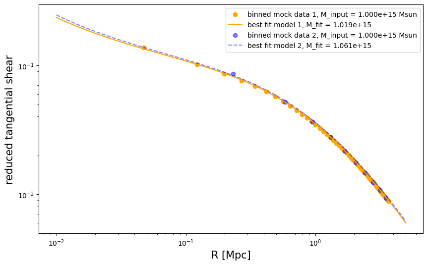
We optimize to find the best-fit mass for the data under the two radial binning schemes.
from clmm.support.sampler import samplers
Note: The samplers[‘minimize’] is a local optimization function, so it does not guarantee to give consistent results (logm_est1 and logm_est2) for all logm_0, which is dependent on the np.random.seed(#) set previously. Some choices of np.random.seed(#) (e.g. set # to 1) will output a logm_0 that leads to a much larger logm_est and thus a misbehaving best-fit model. In contrast, the samplers[‘basinhopping’] is a global optimization function, which can give stable results regardless of the initial guesses, logm_0. Since its underlying method is the same as the samplers[‘minimize’], the two functions take the same arguments.
logm_0 = random.uniform(13.0, 17.0, 1)[0]
# logm_est1 = samplers['minimize'](nfw_to_shear_profile, logm_0,args=[r1, gt_profile1, z1])[0]
logm_est1 = samplers["basinhopping"](
    nfw_to_shear_profile, logm_0, minimizer_kwargs={"args": ([r1, gt_profile1, z1])}
)[0]

# logm_est2 = samplers['minimize'](nfw_to_shear_profile, logm_0,args=[r2, gt_profile2, z2])[0]
logm_est2 = samplers["basinhopping"](
    nfw_to_shear_profile, logm_0, minimizer_kwargs={"args": ([r2, gt_profile2, z2])}
)[0]

m_est1 = 10.0**logm_est1
m_est2 = 10.0**logm_est2

print((m_est1, m_est2))
/tmp/ipykernel_2160586/3502670224.py:3: DeprecationWarning: Conversion of an array with ndim > 0 to a scalar is deprecated, and will error in future. Ensure you extract a single element from your array before performing this operation. (Deprecated NumPy 1.25.)
  m = float(10.0**logm)
(1019206578091240.5, 1060937922400428.9)
Next, we calculate the reduced tangential shear predicted by the two models.
rr = np.logspace(-2, np.log10(5), 100)

gt_model1 = clmm.compute_reduced_tangential_shear(
    rr, m_est1, concentration, cluster_z, src_z, cosmo, delta_mdef=200, halo_profile_model="nfw"
)

gt_model2 = clmm.compute_reduced_tangential_shear(
    rr, m_est2, concentration, cluster_z, src_z, cosmo, delta_mdef=200, halo_profile_model="nfw"
)
We visualize the two predictions of reduced tangential shear.
fig = plt.figure(figsize=(10, 6))

fig.gca().scatter(
    r1, gt_profile1, color="orange", label="binned mock data 1, M_input = %.3e Msun" % cluster_m
)
fig.gca().plot(rr, gt_model1, color="orange", label="best fit model 1, M_fit = %.3e" % m_est1)

fig.gca().scatter(
    r2,
    gt_profile2,
    color="blue",
    alpha=0.5,
    label="binned mock data 2, M_input = %.3e Msun" % cluster_m,
)
fig.gca().plot(
    rr,
    gt_model2,
    color="blue",
    linestyle="--",
    alpha=0.5,
    label="best fit model 2, M_fit = %.3e" % m_est2,
)

plt.semilogx()
plt.semilogy()

plt.legend()
plt.xlabel("R [Mpc]", fontsize=fsize)
plt.ylabel("reduced tangential shear", fontsize=fsize)
Text(0, 0.5, 'reduced tangential shear')