Using the cosmoDC2 catalog
Note: this notebook was produced using a previous version of CLMM (v1.5.1)
Basic usage of the cosmoDC2 extragalactic catalog with CLMM
This notebook can be run at NERSC or CC-IN2P3 where the DESC DC2 products are stored. You need to be a DESC member to be able to access those.
import matplotlib.pyplot as plt
import numpy as np
from astropy.table import Table
import GCRCatalogs
try: import clmm
except:
    import notebook_install
    notebook_install.install_clmm_pipeline(upgrade=False)
    import clmm
Check what version we’re using
clmm.__version__
'1.5.1'
1. Prepare a CLMM GalaxyCluster object from cosmoDC2
Read in the extragalactic catalog cosmoDC2
extragalactic_cat = GCRCatalogs.load_catalog('cosmoDC2_v1.1.4_small')
# Make a CLMM cosmology object from the DC2 cosmology
dc2_cosmo = extragalactic_cat.cosmology
cosmo = clmm.Cosmology(H0 = dc2_cosmo.H0.value, Omega_dm0=dc2_cosmo.Om0-dc2_cosmo.Ob0, Omega_b0=dc2_cosmo.Ob0)
cosmo
<clmm.cosmology.ccl.CCLCosmology at 0x15551392c850>
Get the list of halos with M > mmin in the redshift range [zmin, zmax]
%%time
# get list of massive halos in a given redshift and mass range
mmin = 5.e14 # Msun
zmin = 0.3
zmax = 0.4

massive_halos = extragalactic_cat.get_quantities(
    ['halo_mass','hostHaloMass','redshift','ra', 'dec', 'halo_id'],
    filters=[f'halo_mass > {mmin}','is_central==True',
             f'redshift>{zmin}', f'redshift<{zmax}'])
N_cl = len(massive_halos['halo_mass'])
print(f'There are {N_cl} clusters in this mass and redshift range')
There are 4 clusters in this mass and redshift range
CPU times: user 2.26 s, sys: 9.63 s, total: 11.9 s
Wall time: 1min 54s
Check the units of halo masses in the catalog
We have filtered the catalog using the halo_mass field. There are
two related fields in the catalog: halo_mass and hostHaloMass.
In the cosmoDC2 preprint, Table 2
in appendix B mentions the halo mass to be in units of
M\(_{\odot}\; h^{-1}\). However, the SCHEMA
cosmoDC2
mentions M\(_{\odot}\) for halo_mass. Below, we see that
halo_mass equals hostHaloMass/h. Sohalo_mass is indeed in
units of M\(_{\odot}\), while hostHaloMass is in
M\(_{\odot}\; h^{-1}\).
print(f"hostHaloMass:   {massive_halos['hostHaloMass']}")
print(f"hostHaloMass/h: {massive_halos['hostHaloMass']/cosmo['h']}")
print(f"halo_mass:      {massive_halos['halo_mass']}")
hostHaloMass:   [4.11498904e+14 4.51343114e+14 4.28283670e+14 3.59993019e+14]
hostHaloMass/h: [5.79575921e+14 6.35694527e+14 6.03216436e+14 5.07032421e+14]
halo_mass:      [5.79575921e+14 6.35694527e+14 6.03216436e+14 5.07032421e+14]
Below, we use halo_mass.
Select the most massive one
# Selecting the most massive one

select = massive_halos['halo_mass'] == np.max(massive_halos['halo_mass'])

ra_cl = massive_halos['ra'][select][0]
dec_cl = massive_halos['dec'][select][0]
z_cl = massive_halos['redshift'][select][0]
mass_cl =massive_halos['halo_mass'][select][0]
id_cl = massive_halos['halo_id'][select][0]

print (f'The most massive cluster is halo {id_cl} in ra = {ra_cl:.2f} deg, dec = {dec_cl:.2f} deg, z = {z_cl:.2f}, with mass = {mass_cl:.2e} Msun')
The most massive cluster is halo 95600097373 in ra = 64.26 deg, dec = -34.47 deg, z = 0.32, with mass = 6.36e+14 Msun
Apply coordinates, redshift and magnitude cuts to select backgroud galaxies around the cluster
Box of 0.6 deg around the cluster center
Galaxies with z > z_cluster + 0.1
Galaxies with mag_i < 25
Here, we’re directly gathering the shear components \(\gamma_{1,2}\)
and the convergence \(\kappa\) from the cosmoDC2 catalog. See the
DC2_gt_profiles notebook to see how to also use the intrinsic
ellipticities of the galaxies to compute observed ellipticities
including intrinsic and shear components.
%%time
ra_min, ra_max = ra_cl - 0.3, ra_cl + 0.3
dec_min, dec_max = dec_cl - 0.3, dec_cl + 0.3
z_min = z_cl + 0.1
mag_i_max = 25

coord_filters = [
    'ra >= {}'.format(ra_min),
    'ra < {}'.format(ra_max),
    'dec >= {}'.format(dec_min),
    'dec < {}'.format(dec_max)]
z_filters = ['redshift >= {}'.format(z_min)]
mag_filters = ['mag_i < {}'.format(mag_i_max)]

gal_cat = extragalactic_cat.get_quantities(
    ['galaxy_id', 'ra', 'dec', 'shear_1', 'shear_2',
        'redshift', 'convergence'],
    filters=(coord_filters + z_filters + mag_filters))
CPU times: user 23.1 s, sys: 25.6 s, total: 48.7 s
Wall time: 2min 56s
To compute a reduced tangential shear profile using CLMM, we first need to transform the shear into ellipticities.
The CLMM function
convert_shapes_to_epsilonconvert any shape measurements into the corresponding ellipticities (\(\epsilon\) definition).Then, we build the astropy table of the galaxy catalog that will be used to instantiate a CLMM GalaxyCluster object.
e1, e2 = clmm.utils.convert_shapes_to_epsilon(gal_cat['shear_1'],gal_cat['shear_2'],\
                                              shape_definition='shear',kappa=gal_cat['convergence'])

#store the results into an CLMM GCData (currently it's simply an astropy table)
dat = clmm.GCData(
    [gal_cat['ra'], gal_cat['dec'], e1, e2,
         gal_cat['redshift'], gal_cat['galaxy_id']],
    names=('ra','dec', 'e1', 'e2', 'z','id'))
cl = clmm.GalaxyCluster(str(id_cl), ra_cl, dec_cl, z_cl, dat)
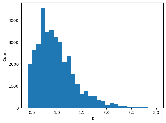
# Quick check of the redshift distribution of the galaxies in the catalog

print(f'Number of galaxies in the catalog: Ngal = {len(cl.galcat)}')
plt.hist(cl.galcat['z'], bins=30);
plt.xlabel('z')
plt.ylabel('Count')
Number of galaxies in the catalog: Ngal = 36403
Text(0, 0.5, 'Count')
2. Use CLMM to compute the reduced tangential shear profile
Compute the tangential and cross shear profiles
NB: Check out the demo_dataops notebook to see examples of all
available options of the functions below.
bin_edges = clmm.dataops.make_bins(0.15, 10, 15, method='evenlog10width') # in Mpc
cl.compute_tangential_and_cross_components(geometry="flat")
cl.make_radial_profile("Mpc", bins=bin_edges,cosmo=cosmo, add=True, include_empty_bins=False, gal_ids_in_bins=False)
pass
3. Sanity check: use CLMM to compute the corresponding NFW model, given the halo mass
The mass definition used in cosmoDC2 is the friend-of-friend mass with linking length b=0.168. In CLMM, the default mass definition is \(M_{200,m}\): it uses an overdensity parameter \(\Delta=200\) with respect to the matter density. Here, we are directly using \(M_{\rm fof}\) in the modeling functions of CLMM, which is inconsistent. However, the goal here is to check that model and data are roughly in agreement.
The model should take into account the redshift distribution of the background galaxies. Here, we simply use the average redshift of the galaxy catalog as this is a quick sanity check that things behave as expected.
For the model, we use a concentration \(c = 4\).
The error bars on the data computed by
make_radial_profilesimply corresponds to the standard error of the mean in the bin (\(\sigma_{\rm bin}/\sqrt{N_{\rm gal\_in\_bin}}\)).
concentration = 4.
reduced_shear = clmm.compute_reduced_tangential_shear(cl.profile['radius'], mass_cl,
                                                      concentration ,z_cl, cl.profile['z'], cosmo,
                                                      halo_profile_model='nfw')
plt.errorbar(cl.profile['radius'],cl.profile['gt'],yerr=cl.profile['gt_err'], label='measured profile')
plt.plot(cl.profile['radius'],reduced_shear, label='model shear')
plt.legend()
plt.xscale('log')
plt.yscale('log')
plt.xlabel('R (Mpc)')
plt.ylabel(r'Reduced shear $\langle g_t\rangle$')
Text(0, 0.5, 'Reduced shear $\langle g_t\rangle$')
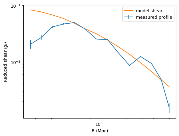
Data and model are in rough agreement at large radii. In the inner region, the lack of resolution of the DC2 simulations yield an unphysical attenuation of the signal. This was remarked upon in the cosmoDC2 paper in the context of galaxy-galaxy lensing.