Example 1b: Impact of miscentering
Fit halo mass to shear profile ivestigating the impact of miscentering on shear profiles
the LSST-DESC CLMM team
This notebook demonstrates the impact of taking wrong cluster centers to
construct and derive the mass from reduced shear profiles
withCLMM. This notebook is based on notebook
“demo_dataops_functionality.ipynb”.
import matplotlib.pyplot as plt
import clmm
import clmm.dataops
from clmm.dataops import compute_tangential_and_cross_components, make_radial_profile, make_bins
from clmm.galaxycluster import GalaxyCluster
import clmm.utils as u
from clmm import Cosmology
from clmm.support import mock_data as mock
import clmm.galaxycluster as gc
from numpy import random
import numpy as np
import clmm.dataops as da
from clmm.support.sampler import fitters

from astropy.coordinates import SkyCoord
import astropy.units as u
Make sure we know which version we’re using
clmm.__version__
'1.12.0'
Define cosmology object
mock_cosmo = Cosmology(H0=70.0, Omega_dm0=0.27 - 0.045, Omega_b0=0.045, Omega_k0=0.0)
np.random.seed(11)
1. Generate cluster objects from mock data
In this example, the mock data only include galaxies drawn from redshift distribution.
Define toy cluster parameters for mock data generation
cosmo = mock_cosmo
cluster_id = "Awesome_cluster"
cluster_m = 1.0e15
cluster_z = 0.3
concentration = 4
ngal_density = 50  # gal/arcmin2
cluster_ra = 20.0
cluster_dec = 40.0
zsrc_min = cluster_z + 0.1  # we only want to draw background galaxies
field_size = 20  # Mpc

ideal_data_z = mock.generate_galaxy_catalog(
    cluster_m,
    cluster_z,
    concentration,
    cosmo,
    "chang13",
    delta_so=200,
    massdef="mean",
    zsrc_min=zsrc_min,
    ngal_density=ngal_density,
    cluster_ra=cluster_ra,
    cluster_dec=cluster_dec,
    field_size=field_size,
)
We want to load this mock data into several CLMM cluster objects, with
cluster centers located in a 0.4 x 0.4 degrees windows around the
original cluster position (cluster_ra, cluster_dec). The user can
change the number of cluster centers if desired. We set the first center
to (cluster_ra,cluster_dec) for comparison reasons, which
corresponds to a == 0 in the cell below.
center_number = 5
cluster_list = []
coord = []

for a in range(0, center_number):
    if a == 0:
        cluster_ra_new = cluster_ra
        cluster_dec_new = cluster_dec
    else:
        cluster_ra_new = random.uniform(cluster_ra - 0.2, cluster_ra + 0.2)
        cluster_dec_new = random.uniform(cluster_dec - 0.2, cluster_dec + 0.2)

    cl = clmm.GalaxyCluster(cluster_id, cluster_ra_new, cluster_dec_new, cluster_z, ideal_data_z)

    print(f"Cluster info = ID: {cl.unique_id}; ra: {cl.ra:.2f}; dec: {cl.dec:.2f}; z_l: {cl.z}")
    print(f"The number of source galaxies is : {len(cl.galcat)}")

    cluster_list.append(cl)
    coord.append(SkyCoord(cl.ra * u.deg, cl.dec * u.deg))
Cluster info = ID: Awesome_cluster; ra: 20.00; dec: 40.00; z_l: 0.3
The number of source galaxies is : 237965
Cluster info = ID: Awesome_cluster; ra: 19.83; dec: 40.09; z_l: 0.3
The number of source galaxies is : 237965
Cluster info = ID: Awesome_cluster; ra: 20.04; dec: 39.96; z_l: 0.3
The number of source galaxies is : 237965
Cluster info = ID: Awesome_cluster; ra: 19.86; dec: 39.84; z_l: 0.3
The number of source galaxies is : 237965
Cluster info = ID: Awesome_cluster; ra: 20.13; dec: 39.83; z_l: 0.3
The number of source galaxies is : 237965
# Offset of the different cluster centers from the position 0,0 (in degree)
offset = [coord[0].separation(coord[i]).value for i in range(5)]
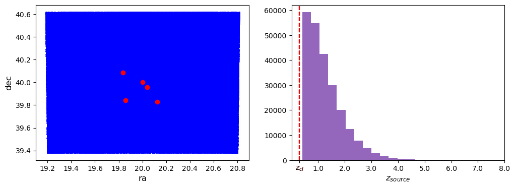
2. Basic checks and plots
galaxy positions
redshift distribution
For a better visualization, we plot all the different cluster centers, represented by the red dots.
f, ax = plt.subplots(1, 2, figsize=(12, 4))

for cl in cluster_list:
    ax[0].scatter(cl.galcat["ra"], cl.galcat["dec"], color="blue", s=1, alpha=0.3)
    ax[0].plot(cl.ra, cl.dec, "ro")
    ax[0].set_ylabel("dec", fontsize="large")
    ax[0].set_xlabel("ra", fontsize="large")

    hist = ax[1].hist(cl.galcat["z"], bins=20)[0]

    ax[1].axvline(cl.z, c="r", ls="--")
    ax[1].set_xlabel("$z_{source}$", fontsize="large")
    xt = {t: f"{t}" for t in ax[1].get_xticks() if t != 0}
    xt[cl.z] = "$z_{cl}$"
    xto = sorted(list(xt.keys()) + [cl.z])
    ax[1].set_xticks(xto)
    ax[1].set_xticklabels(xt[t] for t in xto)
    ax[1].get_xticklabels()[xto.index(cl.z)].set_color("red")
    plt.xlim(0, max(xto))

plt.show()
3. Compute the center effect on the shear profiles
Next, we generate the profiles for all the Cluster objects and save the
profiles into a list. We also save the gt, gx, and radius
columns of each profile into lists, so we can make a plot of these
components.
bin_edges = make_bins(0.3, 6, 10)  # We want to specify the same bins for all the centers.

profile_list = []

for cl in cluster_list:
    theta, e_t, e_x = compute_tangential_and_cross_components(
        ra_lens=cl.ra,
        dec_lens=cl.dec,
        ra_source=cl.galcat["ra"],
        dec_source=cl.galcat["dec"],
        shear1=cl.galcat["e1"],
        shear2=cl.galcat["e2"],
    )
    cl.compute_tangential_and_cross_components(add=True)
    cl.make_radial_profile("Mpc", cosmo=cosmo, bins=bin_edges, include_empty_bins=False)
    profile_list.append(cl.profile)
fig = plt.figure(figsize=(10, 6))

for a in range(0, len(profile_list)):
    fig.gca().errorbar(
        profile_list[a]["radius"],
        profile_list[a]["gt"],
        profile_list[a]["gt_err"],
        linestyle="-",
        marker="o",
        label=f'offset = {"{:.2f}".format(offset[a])}°',
    )

plt.xlabel("log(radius)", size=14)
plt.ylabel("gt", size=14)

plt.legend()
plt.show()
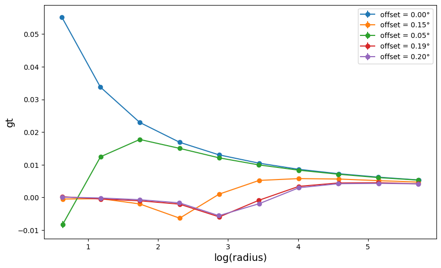
fig2 = plt.figure(figsize=(10, 6))

for a in range(0, len(profile_list)):
    fig2.gca().errorbar(
        profile_list[a]["radius"],
        profile_list[a]["gx"],
        profile_list[a]["gx_err"],
        linestyle="-",
        marker="o",
        label=f'offset = {"{:.2f}".format(offset[a])}°',
    )

plt.xlabel("log(radius)", size=14)
plt.ylabel("gx", size=14)
plt.legend(loc=4)

plt.show()
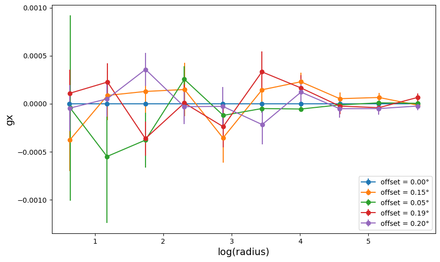
Since we consider GalaxyCluster objects with no shape noise or photo-z
errors, the center (0,0) gives the expected result gx = 0, by
construction. For the other cluster centers, we can see that the cross
shear term average to zero as expected, but the profiles are noisier.
4. Compute the center effect by fitting the Halo mass
In this last step, we compute the fitting Halo mass with the nfw
model and, using a plot, compare the impact of the Cluster centers on
the weak lensing mass.
from clmm.support.sampler import samplers
The function below defines the Halo model. For further information, check the notebook “Example2_Fit_Halo_Mass_to_Shear_Catalog.ipynb”
logm_0 = random.uniform(13.0, 17.0, 1)[0]


def shear_profile_model(r, logm, z_src):
    m = 10.0**logm
    gt_model = clmm.compute_reduced_tangential_shear(
        r, m, concentration, cluster_z, z_src, cosmo, delta_mdef=200, halo_profile_model="nfw"
    )
    return gt_model
for a in range(0, len(cluster_list)):
    popt, pcov = fitters["curve_fit"](
        lambda r, logm: shear_profile_model(r, logm, profile_list[a]["z"]),
        profile_list[a]["radius"],
        profile_list[a]["gt"],
        profile_list[a]["gt_err"],
        bounds=[13.0, 17.0],
    )

    m_est1 = 10.0 ** popt[0]
    m_est_err1 = (
        m_est1 * np.sqrt(pcov[0][0]) * np.log(10)
    )  # convert the error on logm to error on m

    print(f"The fitted mass is : {m_est1:.2e}, for the offset distance: {offset[a]:.2f} deg")
    plt.errorbar(
        offset[a], m_est1, yerr=m_est_err1, fmt=".", color="black", markersize=10
    )  # , label=f'Offset:{"{:.2f}".format(offset[a])}°')

plt.xlabel("offset [deg]", size=12)
plt.ylabel("fitted mass $M_{200,m}$ [M$_{\odot}$]", size=12)
plt.yscale("log")
plt.ylim([5.0e12, 2.0e15])
plt.axhline(cluster_m, label="input mass")
plt.legend(loc="best")
plt.show()
The fitted mass is : 8.75e+14, for the offset distance: 0.00 deg
The fitted mass is : 4.05e+14, for the offset distance: 0.15 deg
The fitted mass is : 8.27e+14, for the offset distance: 0.05 deg
The fitted mass is : 1.24e+14, for the offset distance: 0.19 deg
The fitted mass is : 9.70e+13, for the offset distance: 0.20 deg
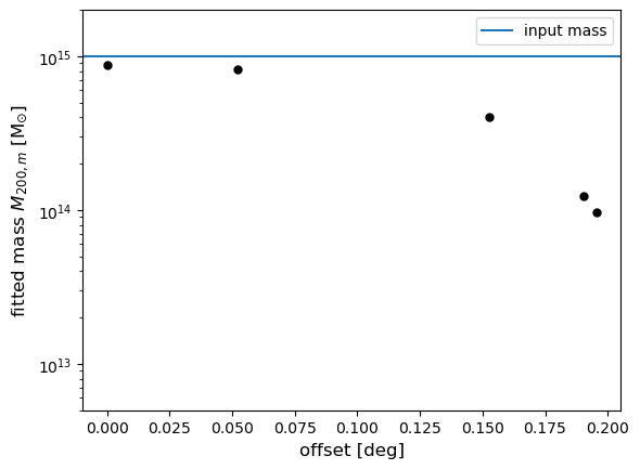
We can see that for cluster centers differing from (0,0), we have a negative effect on the lensing mass, which increases with the offset distance.