Mass conversion between different mass definitions
Mass conversion between spherical overdensity mass definitions
In this notebook, we demonstrates how to convert the mass and concentration between various mass definitions (going from \(200m\) to \(500c\) in this example), and related functionalities, using both the object-oriented and functional interfaces of the code.
import os

os.environ[
    "CLMM_MODELING_BACKEND"
] = "ccl"  # here you may choose ccl, nc (NumCosmo) or ct (cluster_toolkit)
import clmm
import numpy as np
import matplotlib.pyplot as plt
We define a cosmology first:
cosmo = clmm.Cosmology(H0=70.0, Omega_dm0=0.27 - 0.045, Omega_b0=0.045, Omega_k0=0.0)
Create a CLMM Modeling object
Define a mass profile for a given SOD definition
We define halo parameters following the \(200m\) overdensity definition: 1. the mass \(M_{200m}\) 2. the concentration \(c_{200m}\)
# first SOD definition
M1 = 1e14
c1 = 3
massdef1 = "mean"
delta_mdef1 = 200
# cluster redshift
z_cl = 0.4
# create a clmm Modeling object for each profile parametrisation
nfw_def1 = clmm.Modeling(massdef=massdef1, delta_mdef=delta_mdef1, halo_profile_model="nfw")
her_def1 = clmm.Modeling(massdef=massdef1, delta_mdef=delta_mdef1, halo_profile_model="hernquist")
ein_def1 = clmm.Modeling(massdef=massdef1, delta_mdef=delta_mdef1, halo_profile_model="einasto")

# set the properties of the profiles
nfw_def1.set_mass(M1)
nfw_def1.set_concentration(c1)
nfw_def1.set_cosmo(cosmo)

her_def1.set_mass(M1)
her_def1.set_concentration(c1)
her_def1.set_cosmo(cosmo)

ein_def1.set_mass(M1)
ein_def1.set_concentration(c1)
ein_def1.set_cosmo(cosmo)
Compute the enclosed mass in a given radius
Calculate the enclosed masses within r with the class method
eval_mass_in_radius. The calculation can also be done in the
functional interface with compute_profile_mass_in_radius.
The enclosed mass is calculated as
where \(f(x)\) for the different models are
\(\text{NFW}:\quad \ln(1+x)-\frac{x}{1+x}\)
\(\text{Einasto}:\quad \gamma\left(\frac{3}{\alpha}, \frac{2}{\alpha}x^{\alpha}\right)\quad \; (\gamma\text{ is the lower incomplete gamma function},\; \alpha\text{ is the index of the Einasto profile})\)
\(\text{Hernquist}:\quad \left(\frac{x}{1+x}\right)^2\)
r = np.logspace(-2, 0.4, 100)
# object oriented
nfw_def1_enclosed_oo = nfw_def1.eval_mass_in_radius(r3d=r, z_cl=z_cl)
her_def1_enclosed_oo = her_def1.eval_mass_in_radius(r3d=r, z_cl=z_cl)
ein_def1_enclosed_oo = ein_def1.eval_mass_in_radius(r3d=r, z_cl=z_cl)

# functional
nfw_def1_enclosed = clmm.compute_profile_mass_in_radius(
    r3d=r,
    redshift=z_cl,
    cosmo=cosmo,
    mdelta=M1,
    cdelta=c1,
    massdef=massdef1,
    delta_mdef=delta_mdef1,
    halo_profile_model="nfw",
)
her_def1_enclosed = clmm.compute_profile_mass_in_radius(
    r3d=r,
    redshift=z_cl,
    cosmo=cosmo,
    mdelta=M1,
    cdelta=c1,
    massdef=massdef1,
    delta_mdef=delta_mdef1,
    halo_profile_model="hernquist",
)
ein_def1_enclosed = clmm.compute_profile_mass_in_radius(
    r3d=r,
    redshift=z_cl,
    cosmo=cosmo,
    mdelta=M1,
    cdelta=c1,
    massdef=massdef1,
    delta_mdef=delta_mdef1,
    halo_profile_model="einasto",
    alpha=ein_def1.get_einasto_alpha(z_cl),
)
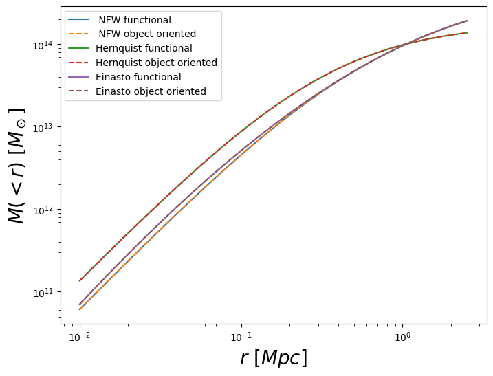
Sanity check: comparison of the results given by the object-oriented and functional interface
fig = plt.figure(figsize=(8, 6))
fig.gca().loglog(r, nfw_def1_enclosed, label=" NFW functional")
fig.gca().loglog(r, nfw_def1_enclosed_oo, ls="--", label=" NFW object oriented")
fig.gca().loglog(r, her_def1_enclosed, label="Hernquist functional")
fig.gca().loglog(r, her_def1_enclosed_oo, ls="--", label="Hernquist object oriented")
fig.gca().loglog(r, ein_def1_enclosed, label="Einasto functional")
fig.gca().loglog(r, ein_def1_enclosed_oo, ls="--", label="Einasto object oriented")
fig.gca().set_xlabel(r"$r\ [Mpc]$", fontsize=20)
fig.gca().set_ylabel(r"$M(<r)\ [M_\odot]$", fontsize=20)
fig.gca().legend()
plt.show()
Compute the spherical overdensity radius
We can also compute the spherical overdensity radius, \(r_{200m}\)
with eval_rdelta (resp. compute_rdelta) in the object oriented
(resp. functional) interface as follows:
## OO interface
r200m_oo = nfw_def1.eval_rdelta(z_cl)

# functional interface
r200m = clmm.compute_rdelta(
    mdelta=M1, redshift=z_cl, cosmo=cosmo, massdef=massdef1, delta_mdef=delta_mdef1
)

print(f"r200m_oo = {r200m_oo} Mpc")
print(f"r200m = {r200m} Mpc")
r200m_oo = 1.056418142453307 Mpc
r200m = 1.056418142453307 Mpc
Conversion to another SOD definition (here we choose 500c)
# New SOD definition
massdef2 = "critical"
delta_mdef2 = 500
To find \(M_2\) and \(c_2\) of the second SOD definition, we solve the system of equations: - \(M_{M_1, c_1}(r_1) = M_{M_2, c_2}(r_1)\) - \(M_{M_1, c_1}(r_2) = M_{M_2, c_2}(r_2)\)
where \(M_{M_i, c_i}(r)\) is the mass enclosed within a sphere of radius \(r\) specified by the overdensity mass \(M_i\) and concentration \(c_i\). Here, \(r_i\) is chosen to be the overdensity radius \(r_{\Delta_i}\) of the \(i\)th overdensity definition, which is calculated with
By identifying \(M_{M_i, c_i}(r_i) = M_{\Delta_i}\) we now have two equations with two unknowns, \(M_2\) and \(c_2\): - \(M_1 = M_{M_2, c_2}(r_1)\) - \(M_{M_1, c_1}(r_2) = M_2\)
The conversion can be done by the convert_mass_concentration method
of a modeling object and the output is the mass and concentration in the
second SOD definition.
M2_nfw_oo, c2_nfw_oo = nfw_def1.convert_mass_concentration(
    z_cl=z_cl, massdef=massdef2, delta_mdef=delta_mdef2
)
M2_her_oo, c2_her_oo = her_def1.convert_mass_concentration(
    z_cl=z_cl, massdef=massdef2, delta_mdef=delta_mdef2
)
M2_ein_oo, c2_ein_oo = ein_def1.convert_mass_concentration(
    z_cl=z_cl, massdef=massdef2, delta_mdef=delta_mdef2
)

print(f"NFW: M2 = {M2_nfw_oo:.2e} M_sun, c2 = {c2_nfw_oo:.2f}")
print(f"HER: M2 = {M2_her_oo:.2e} M_sun, c2 = {c2_her_oo:.2f}")
print(f"EIN: M2 = {M2_ein_oo:.2e} M_sun, c2 = {c2_ein_oo:.2f}")
NFW: M2 = 4.33e+13 M_sun, c2 = 1.33
HER: M2 = 6.48e+13 M_sun, c2 = 1.52
EIN: M2 = 4.36e+13 M_sun, c2 = 1.34
Similarly, there is functional interface to do the conversion (only showing it for NFW below)
M2, c2 = clmm.convert_profile_mass_concentration(
    mdelta=M1,
    cdelta=c1,
    redshift=z_cl,
    cosmo=cosmo,
    massdef=massdef1,
    delta_mdef=delta_mdef1,
    halo_profile_model="nfw",
    massdef2=massdef2,
    delta_mdef2=delta_mdef2,
)
print(f"NFW: M2 = {M2_nfw_oo:.2e} M_sun, c2 = {c2_nfw_oo:.2f}")
NFW: M2 = 4.33e+13 M_sun, c2 = 1.33
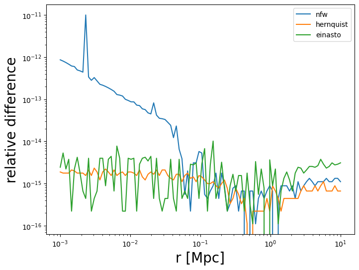
Check conversion by looking at the enclosed mass
To test the conversion method, we plot the relative difference for the enclosed mass between the two mass definitions.
r = np.logspace(-3, 1, 100)
nfw_def2_enclosed = clmm.compute_profile_mass_in_radius(
    r3d=r,
    redshift=z_cl,
    cosmo=cosmo,
    mdelta=M2,
    cdelta=c2,
    massdef=massdef2,
    delta_mdef=delta_mdef2,
    halo_profile_model="nfw",
)
her_def2_enclosed = clmm.compute_profile_mass_in_radius(
    r3d=r,
    redshift=z_cl,
    cosmo=cosmo,
    mdelta=M2_her_oo,
    cdelta=c2_her_oo,
    massdef=massdef2,
    delta_mdef=delta_mdef2,
    halo_profile_model="hernquist",
)
ein_def2_enclosed = clmm.compute_profile_mass_in_radius(
    r3d=r,
    redshift=z_cl,
    cosmo=cosmo,
    mdelta=M2_ein_oo,
    cdelta=c2_ein_oo,
    massdef=massdef2,
    delta_mdef=delta_mdef2,
    halo_profile_model="einasto",
    alpha=ein_def1.get_einasto_alpha(z_cl),
)

fig2 = plt.figure(figsize=(8, 6))
fig2.gca().loglog(
    r, abs(nfw_def2_enclosed / nfw_def1.eval_mass_in_radius(r, z_cl) - 1), ls="-", label="nfw"
)
fig2.gca().loglog(
    r, abs(her_def2_enclosed / her_def1.eval_mass_in_radius(r, z_cl) - 1), ls="-", label="hernquist"
)
fig2.gca().loglog(
    r, abs(ein_def2_enclosed / ein_def1.eval_mass_in_radius(r, z_cl) - 1), ls="-", label="einasto"
)
fig2.gca().set_xlabel("r [Mpc]", fontsize=20)
fig2.gca().set_ylabel(r"relative difference", fontsize=20)
fig2.gca().legend()
plt.show()