Example 5: Using a real datasets (DES)

Fit halo mass to shear profile using DES data

the LSST-DESC CLMM team

This notebook can be run on NERSC.

Here we demonstrate how to run CLMM on real observational datasets. As an example, we use the data from the Dark Energy Survey (DES) public releases. The catalogs can be accessed from the NOIRLab Astro Data Lab.

The steps in this notebook includes: - Setting things up - Selecting a cluster - Downloading the published catalog at the cluster field - Loading the catalog into CLMM - Running CLMM on the dataset

Acknowledgement

DES data: https://des.ncsa.illinois.edu/thanks

Astro Data Lab: https://datalab.noirlab.edu/acknowledgements.php

## 1. Setup

We import packages.

import numpy as np
import matplotlib.pyplot as plt
from astropy.table import Table
import pickle as pkl
from pathlib import Path

## 2. Selecting a cluster

We use the DES Y1 redMaPPer Catalogs (https://des.ncsa.illinois.edu/releases/y1a1/key-catalogs/key-redmapper) to select a list of high-richness (LAMBDA) galaxy clusters, which likely have high masses.

Name	RA (deg)	DEC (deg)	Z_LAMBDA	LAMBDA
RMJ025415.5 585710.7	43.564574	-58.95297	0.429804	234.50368
RMJ051637.4 543001.6	79.155704	-54.500456	0.30416065	195.06956
RMJ224851.8 443106.3	342.215897	-44.518403	0.3514858	178.83827

## 3. Downloading the catalog at the cluster field

We consider RMJ051637.4-543001.6 (ACO S520) as an example. We can access the DES catalog from NOIRLab Data Lab (https://datalab.noirlab.edu/query.php?name=des_dr1.shape_metacal_riz_unblind). No registration is required. We make the query and download the catalogs in “Query Interface”. We use coadd_objects_id to cross match the shape catalog and photo-z catalog (https://datalab.noirlab.edu/query.php?name=des_dr1.photo_z). Since the cluster is at redshift about 0.3, a radius of 0.3 deg would be about a radial distance of 5 Mpc. The final catalog includes shape info and photo-z. Here is an example of the query SQL command. The query could take a few minutes and the size of the catalog is about 1.4 MB (.csv).

SELECT P.mean_z,
C.ra, C.dec, C.e1, C.e2, C.r11, C.r12, C.r21, C.r22
FROM des_dr1.photo_z as P
INNER JOIN des_dr1.shape_metacal_riz_unblind as C
ON P.coadd_objects_id=C.coadd_objects_id
WHERE 't' = Q3C_RADIAL_QUERY(C.ra, C.dec,79.155704, -54.500456, 0.3)
AND P.minchi2<1
AND P.z_sigma<0.1
AND C.flags_select=0

## 4. Loading the catalog into CLMM

Once we have the catalog, we read in the catalog, make cuts on the catalog, and adjust column names to prepare for the analysis in CLMM.

%%time
# Assume the downloaded catalog is at this path:
filename = "ACOS520_DES.csv"
catalog = filename.replace(".csv", ".pkl")
if not Path(catalog).is_file():
    data_0 = Table.read(filename, format="ascii.csv")
    pkl.dump(data_0, open(catalog, "wb"))
else:
    data_0 = pkl.load(open(catalog, "rb"))

CPU times: user 0 ns, sys: 3.52 ms, total: 3.52 ms
Wall time: 3.12 ms

print(data_0.colnames)

['mean_z', 'ra', 'dec', 'e1', 'e2', 'r11', 'r12', 'r21', 'r22']

Shear response

Shears in the DES data have been measured using the metacal method and the catalog provides the shear response terms (\(r11,r22, r12, r21\)) required to calibrate the shear values.

print(np.mean(data_0["r11"]), np.mean(data_0["r22"]))
print(np.mean(data_0["r12"]), np.mean(data_0["r21"]))
r_diag = np.mean([np.mean(data_0["r11"]), np.mean(data_0["r22"])])
r_off_diag = np.mean([np.mean(data_0["r12"]), np.mean(data_0["r21"])])
print(r_diag, r_off_diag, r_off_diag / r_diag)

0.7105854684953065 0.7070498820143473
-0.017056656529555746 0.008455599747631376
0.7088176752548269 -0.004300528390962185 -0.006067185598068083

The diagonal terms are close to each other. The off-diagonal terms are much smaller (<1%). We use the mean of the diagonal terms to reduce noise. We also skip the selection bias since it is typically at percent level.

# Adjust column names.
def adjust_column_names(catalog_in):
    # We consider a map between new and old column names.
    # Note we have considered shear calibration here.
    column_name_map = {
        "ra": "ra",
        "dec": "dec",
        "z": "mean_z",
        "e1": "e1",
        "e2": "e2",
    }

    catalog_out = Table()
    for i in column_name_map:
        catalog_out[i] = catalog_in[column_name_map[i]]

    catalog_out["e1"] /= r_diag
    catalog_out["e2"] /= r_diag

    return catalog_out


obs_galaxies = adjust_column_names(data_0)

select = obs_galaxies["e1"] ** 2 + obs_galaxies["e2"] ** 2 <= 1.0
print(np.sum(~select))
obs_galaxies = obs_galaxies[select]

0

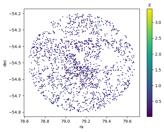
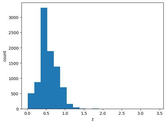
Basic visualization

def make_plots(catalog_in):
    # Scatter plot
    plt.figure()
    plt.scatter(catalog_in["ra"], catalog_in["dec"], c=catalog_in["z"], s=1.0, alpha=1)
    cb = plt.colorbar()
    plt.xlabel("ra")
    plt.ylabel("dec")
    cb.ax.set_title("z")

    # Histogram
    plt.figure()
    plt.hist(catalog_in["z"], bins=20)
    plt.xlabel("z")
    plt.ylabel("count")

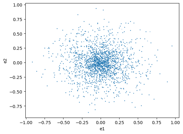
    # Relation
    plt.figure()
    plt.scatter(catalog_in["e1"], catalog_in["e2"], s=1.0, alpha=0.2)
    plt.xlabel("e1")
    plt.ylabel("e2")


make_plots(obs_galaxies)

## 5. Running CLMM on the dataset We use the functions similar to examples/Paper_v1.0/gt_and_use_case.ipynb.

Make a galaxy cluster object

from clmm import Cosmology
import clmm

cosmo = Cosmology(H0=70.0, Omega_dm0=0.27 - 0.045, Omega_b0=0.045, Omega_k0=0.0)

# We consider RMJ051637.4-543001.6 (ACO S520)
cluster_z = 0.30416065  # Cluster redshift
cluster_ra = 79.155704  # Cluster Ra in deg
cluster_dec = -54.500456  # Cluster Dec in deg

# Select background galaxies
obs_galaxies = obs_galaxies[(obs_galaxies["z"] > (cluster_z + 0.1)) & (obs_galaxies["z"] < 1.5)]

obs_galaxies["id"] = np.arange(len(obs_galaxies))

# Put galaxy values on arrays
gal_ra = obs_galaxies["ra"]  # Galaxies Ra in deg
gal_dec = obs_galaxies["dec"]  # Galaxies Dec in deg
gal_e1 = obs_galaxies["e1"]  # Galaxies elipticipy 1
gal_e2 = obs_galaxies["e2"]  # Galaxies elipticipy 2
gal_z = obs_galaxies["z"]  # Galaxies observed redshift
gal_id = obs_galaxies["id"]  # Galaxies ID

# Create a GCData with the galaxies.
galaxies = clmm.GCData(
    [gal_ra, gal_dec, gal_e1, gal_e2, gal_z, gal_id], names=["ra", "dec", "e1", "e2", "z", "id"]
)

# Create a GalaxyCluster.
cluster = clmm.GalaxyCluster("Name of cluster", cluster_ra, cluster_dec, cluster_z, galaxies)

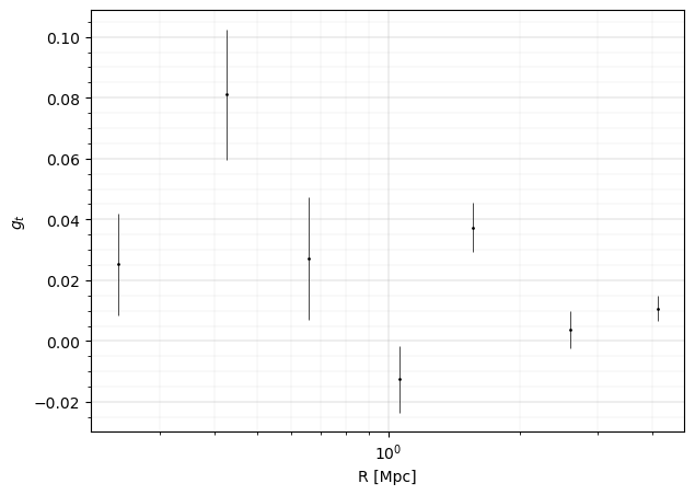
Measure the shear profile

import clmm.dataops as da

# Convert ellipticities into shears for the members.
cluster.compute_tangential_and_cross_components()
print(cluster.galcat.colnames)

# Measure profile and add profile table to the cluster.
cluster.make_radial_profile(
    bins=da.make_bins(0.2, 5.0, 7, method="evenlog10width"),
    bin_units="Mpc",
    cosmo=cosmo,
    include_empty_bins=False,
    gal_ids_in_bins=True,
)
print(cluster.profile.colnames)

['ra', 'dec', 'e1', 'e2', 'z', 'id', 'theta', 'et', 'ex']
['radius_min', 'radius', 'radius_max', 'gt', 'gt_err', 'gx', 'gx_err', 'z', 'z_err', 'n_src', 'W_l', 'gal_id']

fig, ax = plt.subplots(figsize=(7, 5), ncols=1, nrows=1)
errorbar_kwargs = dict(linestyle="", marker="o", markersize=1, elinewidth=0.5, capthick=0.5)
ax.errorbar(
    cluster.profile["radius"],
    cluster.profile["gt"],
    cluster.profile["gt_err"],
    c="k",
    **errorbar_kwargs
)
ax.set_xlabel("R [Mpc]", fontsize=10)
ax.set_ylabel(r"$g_t$", fontsize=10)
ax.set_xscale("log")
ax.grid(lw=0.3)
ax.minorticks_on()
ax.grid(which="minor", lw=0.1)
plt.show()

Theoretical predictions

from clmm.utils import convert_units

# Model relying on the overall redshift distribution of the sources (WtG III Applegate et al. 2014).
z_inf = 1000
concentration = 4.0

bs_mean = np.mean(clmm.utils.compute_beta_s(cluster.galcat["z"], cluster_z, z_inf, cosmo))
bs2_mean = np.mean(clmm.utils.compute_beta_s(cluster.galcat["z"], cluster_z, z_inf, cosmo) ** 2)


def predict_reduced_tangential_shear_redshift_distribution(profile, logm):
    gt = clmm.compute_reduced_tangential_shear(
        r_proj=profile["radius"],  # Radial component of the profile
        mdelta=10**logm,  # Mass of the cluster [M_sun]
        cdelta=concentration,  # Concentration of the cluster
        z_cluster=cluster_z,  # Redshift of the cluster
        z_src=(bs_mean, bs2_mean),  # tuple of (bs_mean, bs2_mean)
        z_src_info="beta",
        approx="order1",
        cosmo=cosmo,
        delta_mdef=200,
        massdef="critical",
        halo_profile_model="nfw",
    )
    return gt


# Model using individual redshift and radial information, to compute the averaged shear in each radial bin, based on the galaxies actually present in that bin.
cluster.galcat["theta_mpc"] = convert_units(
    cluster.galcat["theta"], "radians", "mpc", cluster.z, cosmo
)


def predict_reduced_tangential_shear_individual_redshift(profile, logm):
    return np.array(
        [
            np.mean(
                clmm.compute_reduced_tangential_shear(
                    # Radial component of each source galaxy inside the radial bin
                    r_proj=cluster.galcat[radial_bin["gal_id"]]["theta_mpc"],
                    mdelta=10**logm,  # Mass of the cluster [M_sun]
                    cdelta=concentration,  # Concentration of the cluster
                    z_cluster=cluster_z,  # Redshift of the cluster
                    # Redshift value of each source galaxy inside the radial bin
                    z_src=cluster.galcat[radial_bin["gal_id"]]["z"],
                    cosmo=cosmo,
                    delta_mdef=200,
                    massdef="critical",
                    halo_profile_model="nfw",
                )
            )
            for radial_bin in profile
        ]
    )

Mass fitting

mask_for_fit = cluster.profile["n_src"] > 2
data_for_fit = cluster.profile[mask_for_fit]

from clmm.support.sampler import fitters


def fit_mass(predict_function):
    popt, pcov = fitters["curve_fit"](
        predict_function,
        data_for_fit,
        data_for_fit["gt"],
        data_for_fit["gt_err"],
        bounds=[10.0, 17.0],
    )
    logm, logm_err = popt[0], np.sqrt(pcov[0][0])
    return {
        "logm": logm,
        "logm_err": logm_err,
        "m": 10**logm,
        "m_err": (10**logm) * logm_err * np.log(10),
    }

%%time
fit_redshift_distribution = fit_mass(predict_reduced_tangential_shear_redshift_distribution)
fit_individual_redshift = fit_mass(predict_reduced_tangential_shear_individual_redshift)

CPU times: user 258 ms, sys: 1.15 ms, total: 259 ms
Wall time: 259 ms

print(
    "Best fit mass for N(z) model                     ="
    f' {fit_redshift_distribution["m"]:.3e} +/- {fit_redshift_distribution["m_err"]:.3e} Msun'
)
print(
    "Best fit mass for individual redshift and radius ="
    f' {fit_individual_redshift["m"]:.3e} +/- {fit_individual_redshift["m_err"]:.3e} Msun'
)

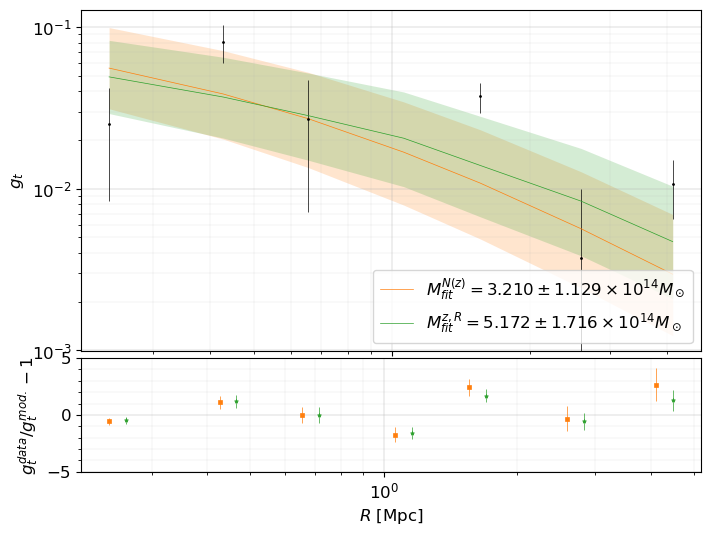
Best fit mass for N(z) model                     = 3.210e+14 +/- 1.129e+14 Msun
Best fit mass for individual redshift and radius = 5.172e+14 +/- 1.716e+14 Msun

Visualization of the results

def get_predicted_shear(predict_function, fit_values):
    gt_est = predict_function(data_for_fit, fit_values["logm"])
    gt_est_err = [
        predict_function(data_for_fit, fit_values["logm"] + i * fit_values["logm_err"])
        for i in (-3, 3)
    ]
    return gt_est, gt_est_err


gt_redshift_distribution, gt_err_redshift_distribution = get_predicted_shear(
    predict_reduced_tangential_shear_redshift_distribution, fit_redshift_distribution
)
gt_individual_redshift, gt_err_individual_redshift = get_predicted_shear(
    predict_reduced_tangential_shear_individual_redshift, fit_individual_redshift
)

chi2_redshift_distribution_dof = np.sum(
    (gt_redshift_distribution - data_for_fit["gt"]) ** 2 / (data_for_fit["gt_err"]) ** 2
) / (len(data_for_fit) - 1)
chi2_individual_redshift_dof = np.sum(
    (gt_individual_redshift - data_for_fit["gt"]) ** 2 / (data_for_fit["gt_err"]) ** 2
) / (len(data_for_fit) - 1)

print(f"Reduced chi2 (N(z) model) = {chi2_redshift_distribution_dof}")
print(f"Reduced chi2 (individual (R,z) model) = {chi2_individual_redshift_dof}")

Reduced chi2 (N(z) model) = 4.780165089363783
Reduced chi2 (individual (R,z) model) = 4.411023500984584

fig, axes = plt.subplots(
    nrows=2,
    ncols=1,
    figsize=(8, 6),
    gridspec_kw={"height_ratios": [3, 1], "wspace": 0.4, "hspace": 0.03},
)

axes[0].errorbar(
    data_for_fit["radius"], data_for_fit["gt"], data_for_fit["gt_err"], c="k", **errorbar_kwargs
)

# Points in grey have not been used for the fit.
axes[0].errorbar(
    cluster.profile["radius"][~mask_for_fit],
    cluster.profile["gt"][~mask_for_fit],
    cluster.profile["gt_err"][~mask_for_fit],
    c="grey",
    **errorbar_kwargs,
)

pow10 = 14
mlabel = lambda name, fits: (
    rf"$M_{{fit}}^{{{name}}} = "
    rf'{fits["m"]/10**pow10:.3f}\pm'
    rf'{fits["m_err"]/10**pow10:.3f}'
    rf"\times 10^{{{pow10}}} M_\odot$"
)

# The model for the 1st method.
axes[0].loglog(
    data_for_fit["radius"],
    gt_redshift_distribution,
    "-C1",
    label=mlabel("N(z)", fit_redshift_distribution),
    lw=0.5,
)

axes[0].fill_between(
    data_for_fit["radius"], *gt_err_redshift_distribution, lw=0, color="C1", alpha=0.2
)

# The model for the 2nd method.
axes[0].loglog(
    data_for_fit["radius"],
    gt_individual_redshift,
    "-C2",
    label=mlabel("z,R", fit_individual_redshift),
    lw=0.5,
)
axes[0].fill_between(
    data_for_fit["radius"], *gt_err_individual_redshift, lw=0, color="C2", alpha=0.2
)


axes[0].set_ylabel(r"$g_t$", fontsize=12)
axes[0].legend(fontsize=12, loc=4)
axes[0].set_xticklabels([])
axes[0].tick_params("x", labelsize=12)
axes[0].tick_params("y", labelsize=12)
axes[1].set_ylim(1.0e-3, 0.5)


errorbar_kwargs2 = {k: v for k, v in errorbar_kwargs.items() if "marker" not in k}
errorbar_kwargs2["markersize"] = 3
errorbar_kwargs2["markeredgewidth"] = 0.5

delta = (cluster.profile["radius"][1] / cluster.profile["radius"][0]) ** 0.15


axes[1].errorbar(
    data_for_fit["radius"],
    data_for_fit["gt"] / gt_redshift_distribution - 1,
    yerr=data_for_fit["gt_err"] / gt_redshift_distribution,
    marker="s",
    c="C1",
    **errorbar_kwargs2,
)
errorbar_kwargs2["markersize"] = 3
errorbar_kwargs2["markeredgewidth"] = 0.5

axes[1].errorbar(
    data_for_fit["radius"] * delta,
    data_for_fit["gt"] / gt_individual_redshift - 1,
    yerr=data_for_fit["gt_err"] / gt_individual_redshift,
    marker="*",
    c="C2",
    **errorbar_kwargs2,
)
axes[1].set_xlabel(r"$R$ [Mpc]", fontsize=12)

axes[1].set_ylabel(r"$g_t^{data}/g_t^{mod.}-1$", fontsize=12)
axes[1].set_xscale("log")

axes[1].set_ylim(-5, 5)

axes[1].tick_params("x", labelsize=12)
axes[1].tick_params("y", labelsize=12)

for ax in axes:
    ax.grid(lw=0.3)
    ax.minorticks_on()
    ax.grid(which="minor", lw=0.1)
plt.show()

# Note since we made cuts on the catalog, the redshift distribution of the remaining sources might not be representative.

References

Zuntz J., Sheldon E., Samuroff S., Troxel M. A., Jarvis M., MacCrann N., Gruen D., et al., 2018, MNRAS, 481, 1149. doi:10.1093/mnras/sty2219

Hoyle B., Gruen D., Bernstein G. M., Rau M. M., De Vicente J., Hartley W. G., Gaztanaga E., et al., 2018, MNRAS, 478, 592. doi:10.1093/mnras/sty957

McClintock T., Varga T. N., Gruen D., Rozo E., Rykoff E. S., Shin T., Melchior P., et al., 2019, MNRAS, 482, 1352. doi:10.1093/mnras/sty2711