Measure WL Profiles
Note
All functions in this section can be used passing the explicit arguments but are also internal functions of the cluster object, and should be used as such. They are just explicitely used here for clarity.
Ex:
theta, g_t, g_x = compute_tangential_and_cross_components(ra_lens, dec_lens,
                ra_source, dec_source, shear1, shear2)
should be done by the user as:
theta, g_t, g_x = cl.compute_tangential_and_cross_components()
import matplotlib.pyplot as plt
import numpy as np
import clmm
import clmm.dataops
from clmm.dataops import compute_tangential_and_cross_components, make_radial_profile, make_bins
from clmm.galaxycluster import GalaxyCluster
import clmm.utils as u
from clmm import Cosmology
from clmm.support import mock_data as mock
Make sure we know which version we’re using
clmm.__version__
'1.12.0'
Define random seed for reproducibility
np.random.seed(11)
Define cosmology object
mock_cosmo = Cosmology(H0=70.0, Omega_dm0=0.27 - 0.045, Omega_b0=0.045, Omega_k0=0.0)
1. Generate cluster object from mock data
In this example, the mock data includes: shape noise, galaxies drawn from redshift distribution and photoz errors.
Define toy cluster parameters for mock data generation
cosmo = mock_cosmo
cluster_id = "Awesome_cluster"
cluster_m = 1.0e15
cluster_z = 0.3
concentration = 4
ngals = 10000

cluster_ra = 0.0
cluster_dec = 90.0

zsrc_min = cluster_z + 0.1  # we only want to draw background galaxies

noisy_data_z = mock.generate_galaxy_catalog(
    cluster_m,
    cluster_z,
    concentration,
    cosmo,
    "chang13",
    zsrc_min=zsrc_min,
    shapenoise=0.05,
    photoz_sigma_unscaled=0.05,
    ngals=ngals,
    cluster_ra=cluster_ra,
    cluster_dec=cluster_dec,
)
Loading this into a CLMM cluster object centered on (0,0)
cl = GalaxyCluster(cluster_id, cluster_ra, cluster_dec, cluster_z, noisy_data_z)
2. Load cluster object containing:
Lens properties (ra_l, dec_l, z_l)
Source properties (ra_s, dec_s, e1, e2) ### Note, if loading from mock data, use: cl = gc.GalaxyCluster.load(“GC_from_mock_data.pkl”)
print("Cluster info = ID:", cl.unique_id, "; ra:", cl.ra, "; dec:", cl.dec, "; z_l :", cl.z)
print("The number of source galaxies is :", len(cl.galcat))
Cluster info = ID: Awesome_cluster ; ra: 0.0 ; dec: 90.0 ; z_l : 0.3
The number of source galaxies is : 10000
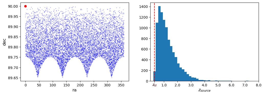
2. Basic checks and plots
galaxy positions
redshift distribution
f, ax = plt.subplots(1, 2, figsize=(12, 4))

ax[0].scatter(cl.galcat["ra"], cl.galcat["dec"], color="blue", s=1, alpha=0.3)
ax[0].plot(cl.ra, cl.dec, "ro")
ax[0].set_ylabel("dec", fontsize="large")
ax[0].set_xlabel("ra", fontsize="large")

hist = ax[1].hist(cl.galcat["z"], bins=40)[0]
ax[1].axvline(cl.z, c="r", ls="--")
ax[1].set_xlabel("$z_{source}$", fontsize="large")
xt = {t: f"{t}" for t in ax[1].get_xticks() if t != 0}
xt[cl.z] = "$z_{cl}$"
xto = sorted(list(xt.keys()) + [cl.z])
ax[1].set_xticks(xto)
ax[1].set_xticklabels(xt[t] for t in xto)
ax[1].get_xticklabels()[xto.index(cl.z)].set_color("red")
plt.xlim(0, max(xto))
plt.show()
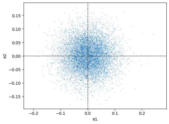
Check ellipticities
fig, ax1 = plt.subplots(1, 1)

ax1.scatter(cl.galcat["e1"], cl.galcat["e2"], s=1, alpha=0.2)
ax1.set_xlabel("e1")
ax1.set_ylabel("e2")
ax1.set_aspect("equal", "datalim")
ax1.axvline(0, linestyle="dotted", color="black")
ax1.axhline(0, linestyle="dotted", color="black")
<matplotlib.lines.Line2D at 0x7f355b172210>
3. Compute and plot shear profiles
3.1 Compute angular separation, cross and tangential shear for each source galaxy
theta, e_t, e_x = compute_tangential_and_cross_components(
    ra_lens=cl.ra,
    dec_lens=cl.dec,
    ra_source=cl.galcat["ra"],
    dec_source=cl.galcat["dec"],
    shear1=cl.galcat["e1"],
    shear2=cl.galcat["e2"],
)
3.1.1 Using GalaxyCluster object
You can also call the function directly from the
GalaxyClusterobjectBy defaut,
compute_tangential_and_cross_componentsuses columns namede1ande2of thegalcattable
cl.compute_tangential_and_cross_components(add=True)
# With the option add the cl object has theta, et and ex new columns
# (default: takes in columns named 'e1' and 'e2' and save the results in 'et' and 'ex')
cl.galcat["et", "ex"].pprint(max_width=-1)
          et                     ex
--------------------- -----------------------
-0.014193669604212844    0.024770292812117598
 0.027593288682813785   -0.031444795110656676
-0.005206908899369735   -0.030510857504521028
  0.11232631436380155     0.07290036434929753
  -0.1256142518002091    0.018802231820255564
 0.019055204201741657     0.06050406041741734
 0.038412781291329155      0.0267416481414113
-0.006667399455776422   -0.016761083213181857
 0.046021962786637574     0.11070669922848506
  0.12516514028251374    -0.06644865696663554
 -0.03582158053386026     0.06837657195958713
 0.050596362016295554   -0.009951128297566936
  0.09421646798534064    0.015587818027871042
  0.07975549313994046    -0.07102831279362883
0.0007749626574570633      0.0478204490885428
-0.028015540528346306     0.04659801344896773
  -0.0529858412338219    0.034872242016200955
 0.038405259482106824    0.026001762081430766
   0.1197017887991115 -0.00017594425025361377
-0.022159728710095222  -0.0005741244288848292
   0.2010969697875847     0.07058694279618334
  -0.0452653271235742    0.005864801263309683
 0.017705557405416968     0.01299156643524062
                  ...                     ...
 0.010719332552569169    -0.13640351684318933
 0.009928255198615999    -0.05882170840311077
-0.015791006414372845   -0.011393464604573304
 0.012215965508645624      0.0049623423240184
 0.004540992199877877    0.017415718137861653
 0.015455418309285786    -0.06012100352723429
  0.02400758201785442      -0.062922003987883
 0.006353797774013829   -0.009676100200072795
 -0.02553419955403451   -0.007604721209673803
 0.036541542133955385    -0.13237962978298412
  0.04922842883460248    0.006502573562270769
  0.04306295121104719    0.009928395972140016
 -0.04534396117336687     0.04809864798978794
  0.13235030069330608    0.010849217743934977
 -0.04648427585274571    -0.05268394123309532
 -0.03498815031434638   -0.001560839875230504
  0.03187266724532606    -0.07335010293675895
  0.06922795072503296    -0.03909067857437158
 0.026474999081928356     0.04501156446867458
  0.06794774688091935     -0.0870781268087891
  0.11658596390772831   -0.007006942480985608
  -0.0582783624179269    -0.01879387705087386
  0.06611775764202141    -0.01725669970366957
Length = 10000 rows
But it’s also possible to choose which columns to use for input and output, e.g. Below we’re storing the results in
e_tanande_crossinstead (explicitely takinge1ande2as input)
cl.compute_tangential_and_cross_components(
    shape_component1="e1",
    shape_component2="e2",
    tan_component="e_tan",
    cross_component="e_cross",
    add=True,
)
cl.galcat["e_tan", "e_cross"].pprint(max_width=-1)
        e_tan                 e_cross
--------------------- -----------------------
-0.014193669604212844    0.024770292812117598
 0.027593288682813785   -0.031444795110656676
-0.005206908899369735   -0.030510857504521028
  0.11232631436380155     0.07290036434929753
  -0.1256142518002091    0.018802231820255564
 0.019055204201741657     0.06050406041741734
 0.038412781291329155      0.0267416481414113
-0.006667399455776422   -0.016761083213181857
 0.046021962786637574     0.11070669922848506
  0.12516514028251374    -0.06644865696663554
 -0.03582158053386026     0.06837657195958713
 0.050596362016295554   -0.009951128297566936
  0.09421646798534064    0.015587818027871042
  0.07975549313994046    -0.07102831279362883
0.0007749626574570633      0.0478204490885428
-0.028015540528346306     0.04659801344896773
  -0.0529858412338219    0.034872242016200955
 0.038405259482106824    0.026001762081430766
   0.1197017887991115 -0.00017594425025361377
-0.022159728710095222  -0.0005741244288848292
   0.2010969697875847     0.07058694279618334
  -0.0452653271235742    0.005864801263309683
 0.017705557405416968     0.01299156643524062
                  ...                     ...
 0.010719332552569169    -0.13640351684318933
 0.009928255198615999    -0.05882170840311077
-0.015791006414372845   -0.011393464604573304
 0.012215965508645624      0.0049623423240184
 0.004540992199877877    0.017415718137861653
 0.015455418309285786    -0.06012100352723429
  0.02400758201785442      -0.062922003987883
 0.006353797774013829   -0.009676100200072795
 -0.02553419955403451   -0.007604721209673803
 0.036541542133955385    -0.13237962978298412
  0.04922842883460248    0.006502573562270769
  0.04306295121104719    0.009928395972140016
 -0.04534396117336687     0.04809864798978794
  0.13235030069330608    0.010849217743934977
 -0.04648427585274571    -0.05268394123309532
 -0.03498815031434638   -0.001560839875230504
  0.03187266724532606    -0.07335010293675895
  0.06922795072503296    -0.03909067857437158
 0.026474999081928356     0.04501156446867458
  0.06794774688091935     -0.0870781268087891
  0.11658596390772831   -0.007006942480985608
  -0.0582783624179269    -0.01879387705087386
  0.06611775764202141    -0.01725669970366957
Length = 10000 rows
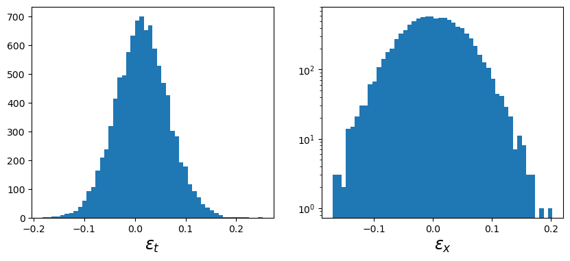
Plot tangential and cross ellipticity distributions for verification, which can be accessed in the galaxy cluster object, cl.
f, ax = plt.subplots(1, 2, figsize=(10, 4))

ax[0].hist(cl.galcat["et"], bins=50)
ax[0].set_xlabel("$\\epsilon_t$", fontsize="xx-large")

ax[1].hist(cl.galcat["ex"], bins=50)
ax[1].set_xlabel("$\\epsilon_x$", fontsize="xx-large")
ax[1].set_yscale("log")
Compute transversal and cross shear profiles in units defined by user, using defaults binning
3.2 Compute shear profile in radial bins
Given the separations in “radians” computed in the previous step, the user may ask for a binned profile in various projected distance units. #### 3.2.1 Default binning - default binning using kpc:
profiles = make_radial_profile(
    [cl.galcat["et"], cl.galcat["ex"], cl.galcat["z"]],
    angsep=cl.galcat["theta"],
    angsep_units="radians",
    bin_units="kpc",
    cosmo=cosmo,
    z_lens=cl.z,
)
# profiles.pprint(max_width=-1)
profiles.show_in_notebook()
| idx | radius_min | radius | radius_max | p_0 | p_0_err | p_1 | p_1_err | p_2 | p_2_err | n_src | weights_sum |
|---|---|---|---|---|---|---|---|---|---|---|---|
| 0 | 49.89926186693261 | 400.9726230192822 | 607.3017710391922 | 0.07369228018322313 | 0.004447742307624298 | 0.006080026121867754 | 0.003603728713525908 | 1.2297028108389079 | 0.051127320754086575 | 166 | 166.0 |
| 1 | 607.3017710391922 | 923.2018463923688 | 1164.7042802114518 | 0.036146516837835 | 0.00227935785688623 | 0.0018176846014553104 | 0.002206990305431071 | 1.229806743651577 | 0.0306826464937024 | 489 | 489.0 |
| 2 | 1164.7042802114518 | 1456.255915260044 | 1722.1067893837112 | 0.02600871899042059 | 0.0018649252714886544 | -0.0021117832844851914 | 0.0017201795943530447 | 1.2904975456410464 | 0.025796286531234478 | 796 | 796.0 |
| 3 | 1722.1067893837112 | 2010.627504774046 | 2279.509298555971 | 0.016452486829944022 | 0.001493469787073072 | -0.0012393150423236211 | 0.0015266379256973623 | 1.2405106399736192 | 0.021870519290172103 | 1104 | 1104.0 |
| 4 | 2279.509298555971 | 2566.5744727945316 | 2836.9118077282305 | 0.015325088325993361 | 0.001347574981311564 | 0.0024568464199461464 | 0.001305269614002815 | 1.249718872885107 | 0.01937972914536564 | 1364 | 1364.0 |
| 5 | 2836.9118077282305 | 3126.4017074551457 | 3394.3143169004898 | 0.010970572729309921 | 0.0012016555444631944 | 0.0017746612850044355 | 0.0011924727814665885 | 1.2654482714997306 | 0.017411676235896328 | 1752 | 1752.0 |
| 6 | 3394.3143169004898 | 3680.361810684402 | 3951.7168260727494 | 0.008230849462521983 | 0.001156373463097785 | 0.00026482017882748204 | 0.0011144802873654758 | 1.2519063116529148 | 0.015901612106466546 | 1972 | 1972.0 |
| 7 | 3951.7168260727494 | 4206.4472560421955 | 4509.119335245009 | 0.00836882393999162 | 0.0013187944446566542 | 0.0020117004045590546 | 0.001347544793784184 | 1.2339023632491457 | 0.018265497762873995 | 1447 | 1447.0 |
| 8 | 4509.119335245009 | 4740.680183376606 | 5066.521844417269 | 0.004837485395708411 | 0.0019128628423446025 | 0.002688253267273817 | 0.001892572870744313 | 1.2803793398548848 | 0.027250788734393197 | 674 | 674.0 |
| 9 | 5066.521844417269 | 5263.692943534735 | 5623.924353589528 | 0.005696398425432691 | 0.003208271061865603 | -0.00011806820317391168 | 0.0031087370020959184 | 1.2520857801069578 | 0.04417548810164287 | 236 | 236.0 |
Note that, because this function bins a generic number of quantities in
the radial profile, its output table names the quantities as p_i and
errors as p_i_err.
3.1.2 Using GalaxyCluster object
The output GCData corresponding to the binning profiled is attached
as a new attribute of the galaxy cluster object.
cl.make_radial_profile("kpc", cosmo=cosmo)
# cl.profile.pprint(max_width=-1)
cl.profile.show_in_notebook()
| idx | radius_min | radius | radius_max | gt | gt_err | gx | gx_err | z | z_err | n_src | W_l |
|---|---|---|---|---|---|---|---|---|---|---|---|
| 0 | 49.89926186693261 | 400.9726230192822 | 607.3017710391922 | 0.07369228018322313 | 0.004447742307624298 | 0.006080026121867754 | 0.003603728713525908 | 1.2297028108389079 | 0.051127320754086575 | 166 | 166.0 |
| 1 | 607.3017710391922 | 923.2018463923688 | 1164.7042802114518 | 0.036146516837835 | 0.00227935785688623 | 0.0018176846014553104 | 0.002206990305431071 | 1.229806743651577 | 0.0306826464937024 | 489 | 489.0 |
| 2 | 1164.7042802114518 | 1456.255915260044 | 1722.1067893837112 | 0.02600871899042059 | 0.0018649252714886544 | -0.0021117832844851914 | 0.0017201795943530447 | 1.2904975456410464 | 0.025796286531234478 | 796 | 796.0 |
| 3 | 1722.1067893837112 | 2010.627504774046 | 2279.509298555971 | 0.016452486829944022 | 0.001493469787073072 | -0.0012393150423236211 | 0.0015266379256973623 | 1.2405106399736192 | 0.021870519290172103 | 1104 | 1104.0 |
| 4 | 2279.509298555971 | 2566.5744727945316 | 2836.9118077282305 | 0.015325088325993361 | 0.001347574981311564 | 0.0024568464199461464 | 0.001305269614002815 | 1.249718872885107 | 0.01937972914536564 | 1364 | 1364.0 |
| 5 | 2836.9118077282305 | 3126.4017074551457 | 3394.3143169004898 | 0.010970572729309921 | 0.0012016555444631944 | 0.0017746612850044355 | 0.0011924727814665885 | 1.2654482714997306 | 0.017411676235896328 | 1752 | 1752.0 |
| 6 | 3394.3143169004898 | 3680.361810684402 | 3951.7168260727494 | 0.008230849462521983 | 0.001156373463097785 | 0.00026482017882748204 | 0.0011144802873654758 | 1.2519063116529148 | 0.015901612106466546 | 1972 | 1972.0 |
| 7 | 3951.7168260727494 | 4206.4472560421955 | 4509.119335245009 | 0.00836882393999162 | 0.0013187944446566542 | 0.0020117004045590546 | 0.001347544793784184 | 1.2339023632491457 | 0.018265497762873995 | 1447 | 1447.0 |
| 8 | 4509.119335245009 | 4740.680183376606 | 5066.521844417269 | 0.004837485395708411 | 0.0019128628423446025 | 0.002688253267273817 | 0.001892572870744313 | 1.2803793398548848 | 0.027250788734393197 | 674 | 674.0 |
| 9 | 5066.521844417269 | 5263.692943534735 | 5623.924353589528 | 0.005696398425432691 | 0.003208271061865603 | -0.00011806820317391168 | 0.0031087370020959184 | 1.2520857801069578 | 0.04417548810164287 | 236 | 236.0 |
You can see that this profile table contains metadata regarding the
comology and bin units
print("Cosmology:", cl.profile.meta["cosmo"])
print("bin units:", cl.profile.meta["bin_units"])
Cosmology: CCLCosmology(H0=70.0, Omega_dm0=0.22500000000000003, Omega_b0=0.045, Omega_k0=0.0)
bin units: kpc
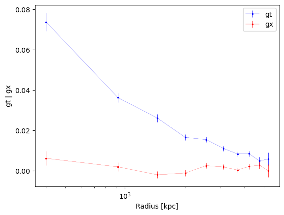
Use function to plot the profiles
fig, ax = cl.plot_profiles(xscale="log")
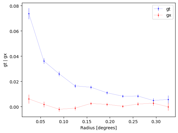
default binning using degrees:
new_profiles = cl.make_radial_profile("degrees", cosmo=cosmo)
fig1, ax1 = cl.plot_profiles()
/global/homes/a/aguena/.local/perlmutter/python-3.11/lib/python3.11/site-packages/clmm-1.12.0-py3.11.egg/clmm/galaxycluster.py:613: UserWarning: overwriting profile table.
3.2.2 User-defined binning
The users may also provide their own binning, in user-defined units, to
compute the transversal and cross shear profiles. The make_bins
function is provided in utils.py and allow for various options.
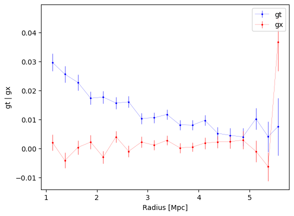
e.g., generate 20 bins between 1 and 6 Mpc, linearly spaced.
new_bins = make_bins(1, 6, nbins=20, method="evenwidth")

# Make the shear profile in this binning
new_profiles = cl.make_radial_profile("Mpc", bins=new_bins, cosmo=cosmo)

fig1, ax1 = cl.plot_profiles()
/global/homes/a/aguena/.local/perlmutter/python-3.11/lib/python3.11/site-packages/clmm-1.12.0-py3.11.egg/clmm/galaxycluster.py:613: UserWarning: overwriting profile table.
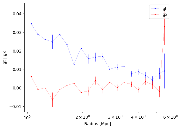
e.g., generate 20 bins between 1 and 6 Mpc, evenly spaced in log space.
new_bins = make_bins(1, 6, nbins=20, method="evenlog10width")

new_profiles = cl.make_radial_profile("Mpc", bins=new_bins, cosmo=cosmo)
fig1, ax1 = cl.plot_profiles()
ax1.set_xscale("log")
/global/homes/a/aguena/.local/perlmutter/python-3.11/lib/python3.11/site-packages/clmm-1.12.0-py3.11.egg/clmm/galaxycluster.py:613: UserWarning: overwriting profile table.
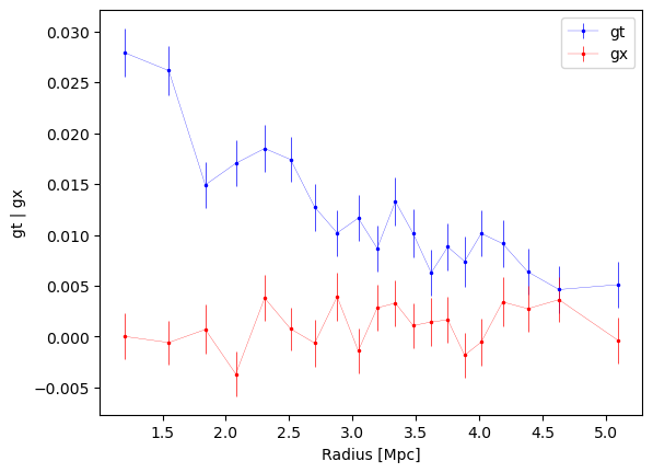
e.g., generate 20 bins between 1 and 6 Mpc, each contaning the same number of galaxies
# First, convert the source separation table to Mpc
seps = u.convert_units(cl.galcat["theta"], "radians", "Mpc", redshift=cl.z, cosmo=cosmo)

new_bins = make_bins(1, 6, nbins=20, method="equaloccupation", source_seps=seps)
new_profiles = cl.make_radial_profile("Mpc", bins=new_bins, cosmo=cosmo)

print(f"number of galaxies in each bin: {list(cl.profile['n_src'])}")
fig1, ax1 = cl.plot_profiles()
number of galaxies in each bin: [477, 477, 476, 477, 476, 477, 476, 477, 476, 477, 477, 476, 477, 476, 477, 476, 477, 476, 477, 477]
/global/homes/a/aguena/.local/perlmutter/python-3.11/lib/python3.11/site-packages/clmm-1.12.0-py3.11.egg/clmm/galaxycluster.py:613: UserWarning: overwriting profile table.
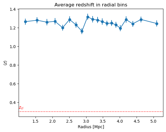
3.2.3 Other individual profile quantities may also be accessed
plt.title("Average redshift in radial bins")
plt.errorbar(new_profiles["radius"], new_profiles["z"], new_profiles["z_err"], marker="o")
plt.axhline(cl.z, linestyle="dotted", color="r")
plt.text(1, cl.z * 1.1, "$z_{cl}$", color="r")
plt.xlabel("Radius [Mpc]")
plt.ylabel("$\langle z\\rangle$")
plt.show()
4. Focus on some options
4.1. gal_ids_in_bins option
adds a gal_id field to the profile GCData. For each bin of the
profile, this is filled with the list of galaxy IDs for the galaxies
that have fallen in that bin.
cl.make_radial_profile("Mpc", cosmo=cosmo, gal_ids_in_bins=True);
/global/homes/a/aguena/.local/perlmutter/python-3.11/lib/python3.11/site-packages/clmm-1.12.0-py3.11.egg/clmm/galaxycluster.py:613: UserWarning: overwriting profile table.
# Here the list of galaxy IDs that are in the first bin of the tangential shear profile
gal_list = cl.profile["gal_id"][0]
print(gal_list)
[30, 132, 180, 184, 190, 268, 346, 369, 433, 542, 553, 791, 822, 988, 1023, 1105, 1113, 1198, 1199, 1205, 1212, 1240, 1281, 1308, 1357, 1607, 1648, 1672, 1741, 1754, 1846, 1907, 1957, 2006, 2014, 2338, 2561, 2618, 2622, 2632, 2719, 2833, 2841, 2856, 2964, 3052, 3062, 3087, 3088, 3096, 3116, 3188, 3324, 3400, 3433, 3551, 3572, 3691, 3694, 3746, 3790, 3849, 3855, 3862, 3878, 3893, 4033, 4037, 4048, 4215, 4236, 4300, 4321, 4344, 4496, 4559, 4562, 4651, 4746, 4889, 4942, 4956, 5073, 5139, 5268, 5294, 5345, 5391, 5608, 5785, 5900, 5925, 5961, 5993, 6025, 6153, 6179, 6218, 6284, 6318, 6322, 6349, 6431, 6610, 6636, 6651, 6701, 6706, 6786, 6802, 6818, 6859, 6963, 6970, 7017, 7079, 7212, 7330, 7376, 7383, 7402, 7415, 7448, 7462, 7489, 7723, 7793, 7870, 7933, 7949, 8023, 8073, 8122, 8137, 8211, 8399, 8501, 8527, 8566, 8653, 8822, 8873, 8879, 8915, 8922, 8937, 9128, 9130, 9138, 9188, 9189, 9252, 9470, 9519, 9589, 9596, 9712, 9749, 9775, 9785, 9804, 9867, 9870, 9943, 9990, 9997]
4.2. User-defined naming scheme
The user may specify which columns to use from the galcat table to
perform the binned average. If none is specified, the code looks for
columns names et and ex. Below, we average in bins the
columnse_tan and e_cross of galcat and store the results
in the columns g_tan and g_cross of the profile table of the
cluster object.
cl.make_radial_profile(
    "kpc",
    cosmo=cosmo,
    tan_component_in="e_tan",
    cross_component_in="e_cross",
    tan_component_out="g_tan",
    cross_component_out="g_cross",
)
# cl.profile.pprint(max_width=-1)
cl.profile.show_in_notebook()
/global/homes/a/aguena/.local/perlmutter/python-3.11/lib/python3.11/site-packages/clmm-1.12.0-py3.11.egg/clmm/galaxycluster.py:613: UserWarning: overwriting profile table.
| idx | radius_min | radius | radius_max | g_tan | g_tan_err | g_cross | g_cross_err | z | z_err | n_src | W_l |
|---|---|---|---|---|---|---|---|---|---|---|---|
| 0 | 49.89926186693261 | 400.9726230192822 | 607.3017710391922 | 0.07369228018322313 | 0.004447742307624298 | 0.006080026121867754 | 0.003603728713525908 | 1.2297028108389079 | 0.051127320754086575 | 166 | 166.0 |
| 1 | 607.3017710391922 | 923.2018463923688 | 1164.7042802114518 | 0.036146516837835 | 0.00227935785688623 | 0.0018176846014553104 | 0.002206990305431071 | 1.229806743651577 | 0.0306826464937024 | 489 | 489.0 |
| 2 | 1164.7042802114518 | 1456.255915260044 | 1722.1067893837112 | 0.02600871899042059 | 0.0018649252714886544 | -0.0021117832844851914 | 0.0017201795943530447 | 1.2904975456410464 | 0.025796286531234478 | 796 | 796.0 |
| 3 | 1722.1067893837112 | 2010.627504774046 | 2279.509298555971 | 0.016452486829944022 | 0.001493469787073072 | -0.0012393150423236211 | 0.0015266379256973623 | 1.2405106399736192 | 0.021870519290172103 | 1104 | 1104.0 |
| 4 | 2279.509298555971 | 2566.5744727945316 | 2836.9118077282305 | 0.015325088325993361 | 0.001347574981311564 | 0.0024568464199461464 | 0.001305269614002815 | 1.249718872885107 | 0.01937972914536564 | 1364 | 1364.0 |
| 5 | 2836.9118077282305 | 3126.4017074551457 | 3394.3143169004898 | 0.010970572729309921 | 0.0012016555444631944 | 0.0017746612850044355 | 0.0011924727814665885 | 1.2654482714997306 | 0.017411676235896328 | 1752 | 1752.0 |
| 6 | 3394.3143169004898 | 3680.361810684402 | 3951.7168260727494 | 0.008230849462521983 | 0.001156373463097785 | 0.00026482017882748204 | 0.0011144802873654758 | 1.2519063116529148 | 0.015901612106466546 | 1972 | 1972.0 |
| 7 | 3951.7168260727494 | 4206.4472560421955 | 4509.119335245009 | 0.00836882393999162 | 0.0013187944446566542 | 0.0020117004045590546 | 0.001347544793784184 | 1.2339023632491457 | 0.018265497762873995 | 1447 | 1447.0 |
| 8 | 4509.119335245009 | 4740.680183376606 | 5066.521844417269 | 0.004837485395708411 | 0.0019128628423446025 | 0.002688253267273817 | 0.001892572870744313 | 1.2803793398548848 | 0.027250788734393197 | 674 | 674.0 |
| 9 | 5066.521844417269 | 5263.692943534735 | 5623.924353589528 | 0.005696398425432691 | 0.003208271061865603 | -0.00011806820317391168 | 0.0031087370020959184 | 1.2520857801069578 | 0.04417548810164287 | 236 | 236.0 |
The user may also define the name of the output table attribute. Below,
we asked the binned profile to be saved into the
reduced_shear_profile attribute
cl.make_radial_profile(
    "kpc",
    cosmo=cosmo,
    tan_component_in="e_tan",
    cross_component_in="e_cross",
    tan_component_out="g_tan",
    cross_component_out="g_cross",
    table_name="reduced_shear_profile",
)
# cl.reduced_shear_profile.pprint(max_width=-1)
cl.reduced_shear_profile.show_in_notebook()
| idx | radius_min | radius | radius_max | g_tan | g_tan_err | g_cross | g_cross_err | z | z_err | n_src | W_l |
|---|---|---|---|---|---|---|---|---|---|---|---|
| 0 | 49.89926186693261 | 400.9726230192822 | 607.3017710391922 | 0.07369228018322313 | 0.004447742307624298 | 0.006080026121867754 | 0.003603728713525908 | 1.2297028108389079 | 0.051127320754086575 | 166 | 166.0 |
| 1 | 607.3017710391922 | 923.2018463923688 | 1164.7042802114518 | 0.036146516837835 | 0.00227935785688623 | 0.0018176846014553104 | 0.002206990305431071 | 1.229806743651577 | 0.0306826464937024 | 489 | 489.0 |
| 2 | 1164.7042802114518 | 1456.255915260044 | 1722.1067893837112 | 0.02600871899042059 | 0.0018649252714886544 | -0.0021117832844851914 | 0.0017201795943530447 | 1.2904975456410464 | 0.025796286531234478 | 796 | 796.0 |
| 3 | 1722.1067893837112 | 2010.627504774046 | 2279.509298555971 | 0.016452486829944022 | 0.001493469787073072 | -0.0012393150423236211 | 0.0015266379256973623 | 1.2405106399736192 | 0.021870519290172103 | 1104 | 1104.0 |
| 4 | 2279.509298555971 | 2566.5744727945316 | 2836.9118077282305 | 0.015325088325993361 | 0.001347574981311564 | 0.0024568464199461464 | 0.001305269614002815 | 1.249718872885107 | 0.01937972914536564 | 1364 | 1364.0 |
| 5 | 2836.9118077282305 | 3126.4017074551457 | 3394.3143169004898 | 0.010970572729309921 | 0.0012016555444631944 | 0.0017746612850044355 | 0.0011924727814665885 | 1.2654482714997306 | 0.017411676235896328 | 1752 | 1752.0 |
| 6 | 3394.3143169004898 | 3680.361810684402 | 3951.7168260727494 | 0.008230849462521983 | 0.001156373463097785 | 0.00026482017882748204 | 0.0011144802873654758 | 1.2519063116529148 | 0.015901612106466546 | 1972 | 1972.0 |
| 7 | 3951.7168260727494 | 4206.4472560421955 | 4509.119335245009 | 0.00836882393999162 | 0.0013187944446566542 | 0.0020117004045590546 | 0.001347544793784184 | 1.2339023632491457 | 0.018265497762873995 | 1447 | 1447.0 |
| 8 | 4509.119335245009 | 4740.680183376606 | 5066.521844417269 | 0.004837485395708411 | 0.0019128628423446025 | 0.002688253267273817 | 0.001892572870744313 | 1.2803793398548848 | 0.027250788734393197 | 674 | 674.0 |
| 9 | 5066.521844417269 | 5263.692943534735 | 5623.924353589528 | 0.005696398425432691 | 0.003208271061865603 | -0.00011806820317391168 | 0.0031087370020959184 | 1.2520857801069578 | 0.04417548810164287 | 236 | 236.0 |
4.3 Compute a DeltaSigma profile instead of a shear profile
The is_deltasigma option allows the user to return a cross and
tangential \(\Delta\Sigma\) (excess surface density) value for each
galaxy in the catalog, provided galcat contains the redshifts of the
galaxies and provided a cosmology is passed to the function. The columns
DeltaSigma_tan and DeltaSigma_cross are added to the galcat
table.
cl.compute_tangential_and_cross_components(
    shape_component1="e1",
    shape_component2="e2",
    tan_component="DeltaSigma_tan",
    cross_component="DeltaSigma_cross",
    add=True,
    cosmo=cosmo,
    is_deltasigma=True,
)
cl.galcat.columns
/global/homes/a/aguena/.local/perlmutter/python-3.11/lib/python3.11/site-packages/clmm-1.12.0-py3.11.egg/clmm/cosmology/parent_class.py:110: UserWarning:
Some source redshifts are lower than the cluster redshift.
Sigma_crit = np.inf for those galaxies.
<TableColumns names=('ra','dec','e1','e2','z','ztrue','pzpdf','id','theta','et','ex','e_tan','e_cross','sigma_c','DeltaSigma_tan','DeltaSigma_cross')>
The signal-to-noise of a \(\Delta\Sigma\) profile is improved when
applying optimal weights accounting for photoz, shape noise, precision
of the shape measurements. These weights are computed using the
compute_galaxy_weights methods of the GalaxyCluster class, ans
stored as an extra columns of the galcat table (see the
demo_compute_deltasigma_weights notebook).
cl.compute_galaxy_weights(
    use_pdz=True,
    use_shape_noise=True,
    shape_component1="e1",
    shape_component2="e2",
    cosmo=cosmo,
    is_deltasigma=True,
    add=True,
)

cl.galcat.columns
/global/homes/a/aguena/.local/perlmutter/python-3.11/lib/python3.11/site-packages/clmm-1.12.0-py3.11.egg/clmm/cosmology/parent_class.py:110: UserWarning:
Some source redshifts are lower than the cluster redshift.
Sigma_crit = np.inf for those galaxies.
<TableColumns names=('ra','dec','e1','e2','z','ztrue','pzpdf','id','theta','et','ex','e_tan','e_cross','sigma_c','DeltaSigma_tan','DeltaSigma_cross','sigma_c_eff','w_ls')>
Because these operations required a Cosmology, it was added to
galcat metadata:
cl.galcat.meta["cosmo"]
'CCLCosmology(H0=70.0, Omega_dm0=0.22500000000000003, Omega_b0=0.045, Omega_k0=0.0)'
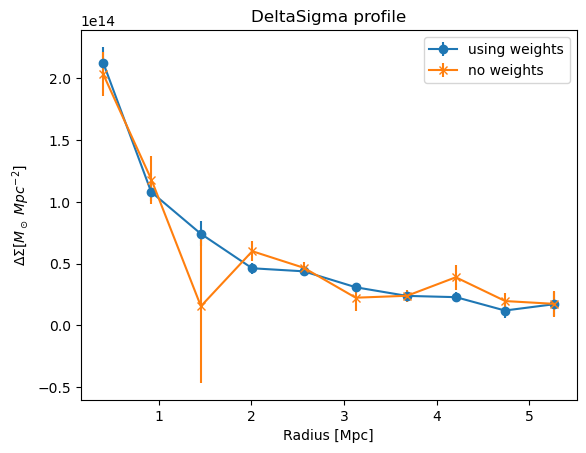
The binned profile is obtained, as before. Below, we use the values
obtained from the previous step to compute the binned profile. The
latter is saved in a new DeltaSigma_profile table of the
GalaxyCluster object. If use_weights=True, the weighted average is
performed using the weights stored in galcat.
"""
cl.make_radial_profile("Mpc", cosmo=cosmo,
                       tan_component_in='DeltaSigma_tan', cross_component_in='DeltaSigma_cross',
                       tan_component_out='DeltaSigma_tan', cross_component_out='DeltaSigma_cross',
                       table_name='DeltaSigma_profile').pprint(max_width=-1)
"""
cl.make_radial_profile(
    "Mpc",
    cosmo=cosmo,
    tan_component_in="DeltaSigma_tan",
    cross_component_in="DeltaSigma_cross",
    tan_component_out="DeltaSigma_tan",
    cross_component_out="DeltaSigma_cross",
    table_name="DeltaSigma_profile",
    use_weights=True,
);
# cl.DeltaSigma_profile.pprint(max_width=-1)
cl.DeltaSigma_profile.show_in_notebook()
| idx | radius_min | radius | radius_max | DeltaSigma_tan | DeltaSigma_tan_err | DeltaSigma_cross | DeltaSigma_cross_err | z | z_err | n_src | W_l |
|---|---|---|---|---|---|---|---|---|---|---|---|
| 0 | 0.04989926186693261 | 0.40181702725631496 | 0.6073017710391921 | 212624096345828.4 | 12655402657482.291 | 15732761567739.193 | 12296182303656.047 | 1.463567191680782 | 0.057677669439307994 | 166 | 3.9434463355203176e-27 |
| 1 | 0.6073017710391921 | 0.91997828958074 | 1.1647042802114518 | 107977347608942.44 | 7146281284443.765 | 7854532242277.562 | 6871295327248.187 | 1.4877929742814777 | 0.03349197273932518 | 489 | 1.1389768721844858e-26 |
| 2 | 1.1647042802114518 | 1.4541808661703517 | 1.722106789383711 | 74201758964831.72 | 10177508339578.314 | -5945024572810.5 | 11944613981983.064 | 1.5363457767152802 | 0.028559938092406267 | 796 | 1.92631612565532e-26 |
| 3 | 1.722106789383711 | 2.009026398675747 | 2.2795092985559706 | 46230165382404.27 | 4653190892495.732 | -3134990325918.112 | 4649628199369.969 | 1.4970067826674796 | 0.024468325558512957 | 1104 | 2.572249004973109e-26 |
| 4 | 2.2795092985559706 | 2.565913261120448 | 2.8369118077282303 | 43758379098921.62 | 4082127758886.9214 | 5693879230724.072 | 3946533113222.4775 | 1.5110619977710178 | 0.02170896089793281 | 1364 | 3.208215057365071e-26 |
| 5 | 2.8369118077282303 | 3.1303364895960697 | 3.3943143169004895 | 30806708059922.51 | 3852954883455.599 | 4681373494567.763 | 3834674599987.0015 | 1.5032833726840107 | 0.018517337757787914 | 1752 | 4.1690647252400884e-26 |
| 6 | 3.3943143169004895 | 3.679064294819914 | 3.951716826072749 | 23886688363580.266 | 3507193605501.202 | -219434498994.54385 | 3416172893642.015 | 1.4964103679695608 | 0.0174998417128246 | 1972 | 4.6712786340082035e-26 |
| 7 | 3.951716826072749 | 4.2081944476143835 | 4.509119335245009 | 22855624279366.89 | 4198818643913.042 | 5320352842195.89 | 4188709345517.6226 | 1.4969016764903824 | 0.020786085574901803 | 1447 | 3.3876100059854263e-26 |
| 8 | 4.509119335245009 | 4.736457929318898 | 5.066521844417268 | 12048101637529.809 | 5702911589032.317 | 9297096328274.348 | 5661409712336.724 | 1.5349261798982219 | 0.029188305071441458 | 674 | 1.616613161376441e-26 |
| 9 | 5.066521844417268 | 5.265782408007491 | 5.623924353589528 | 17132048449502.816 | 9626411199780.172 | -2710585711141.1704 | 9301892446424.824 | 1.4907418293219912 | 0.04783133799403878 | 236 | 5.620502059384091e-27 |
To compare, we make use of the functional interface to compute the
unweighted averaged profile. The outputs columns are called by default
p_0, p_1, etc.
avg_profile_noweights = make_radial_profile(
    [cl.galcat["DeltaSigma_tan"], cl.galcat["DeltaSigma_cross"]],
    cl.galcat["theta"],
    z_lens=cl.z,
    bin_units="Mpc",
    angsep_units="radians",
    cosmo=cosmo,
    weights=None,
)
avg_profile_noweights.columns
<TableColumns names=('radius_min','radius','radius_max','p_0','p_0_err','p_1','p_1_err','n_src','weights_sum')>
plt.errorbar(
    cl.DeltaSigma_profile["radius"],
    cl.DeltaSigma_profile["DeltaSigma_tan"],
    cl.DeltaSigma_profile["DeltaSigma_tan_err"],
    marker="o",
    label="using weights",
)
plt.errorbar(
    avg_profile_noweights["radius"],
    avg_profile_noweights["p_0"],
    avg_profile_noweights["p_0_err"],
    marker="x",
    label="no weights",
)

plt.title("DeltaSigma profile")
plt.xlabel("Radius [Mpc]")
plt.ylabel("$\Delta\Sigma [M_\odot\; Mpc^{-2}]$")
plt.legend()
plt.show()