Model WL Profiles
Notebook for generating an example galaxy cluster model.
This notebook goes through the steps to generate model data for galaxy cluster weak lensing observables. In particular, we define a galaxy cluster model that follows and NFW distribution and generate various profiles for the model (mass density, convergence, shear, etc.), which we plot. Note, a full pipeline to measure a galaxy cluster weak lensing mass requires fitting the observed (or mock) data to a model.
Note 1: This notebook shows how to make this modeling using functions, it is simpler than using an object oriented approach but can also be slower. For the object oriented approach, see demo_theory_functionality_oo.ipynb.
Note 2: There are many different approaches on using the redshift information of the source. For a detailed description on it, see demo_theory_functionality_diff_z_types.ipynb.
import numpy as np
import matplotlib.pyplot as plt

%matplotlib inline
Imports specific to clmm
import os

os.environ[
    "CLMM_MODELING_BACKEND"
] = "ccl"  # here you may choose ccl, nc (NumCosmo) or ct (cluster_toolkit)
import clmm
import clmm.theory as m
from clmm import Cosmology
Make sure we know which version we’re using
clmm.__version__
'1.12.0'
Define a cosmology using astropy
cosmo = Cosmology(H0=70.0, Omega_dm0=0.27 - 0.045, Omega_b0=0.045, Omega_k0=0.0)
Define the galaxy cluster model. Here, we choose parameters that describe the galaxy cluster model, including the mass definition, concentration, and mass distribution. For the mass distribution, we choose a distribution that follows an NFW profile.
# cluster properties
density_profile_parametrization = "nfw"
mass_Delta = 200
cluster_mass = 1.0e15
cluster_concentration = 4
z_cl = 1.0

# source properties
z_src = 2.0  # all sources in the same plan
z_distrib_func = clmm.redshift.distributions.chang2013  # sources redshift following a distribution
alpha = [2, -0.5]
Quick test of all theory functionality
r3d = np.logspace(-2, 2, 100)
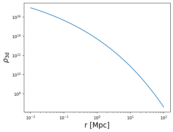
rho = m.compute_3d_density(
    r3d, mdelta=cluster_mass, cdelta=cluster_concentration, z_cl=z_cl, cosmo=cosmo
)
Sigma = m.compute_surface_density(
    r3d,
    cluster_mass,
    cluster_concentration,
    z_cl,
    cosmo=cosmo,
    delta_mdef=mass_Delta,
    halo_profile_model=density_profile_parametrization,
)
DeltaSigma = m.compute_excess_surface_density(
    r3d,
    cluster_mass,
    cluster_concentration,
    z_cl,
    cosmo=cosmo,
    delta_mdef=mass_Delta,
    halo_profile_model=density_profile_parametrization,
)
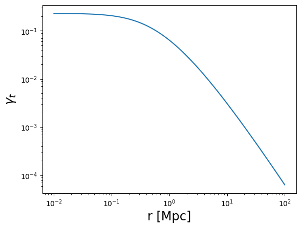
gammat = m.compute_tangential_shear(
    r3d,
    mdelta=cluster_mass,
    cdelta=cluster_concentration,
    z_cluster=z_cl,
    z_src=z_src,
    cosmo=cosmo,
    delta_mdef=mass_Delta,
    halo_profile_model=density_profile_parametrization,
    z_src_info="discrete",
)
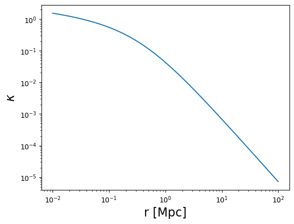
kappa = m.compute_convergence(
    r3d,
    mdelta=cluster_mass,
    cdelta=cluster_concentration,
    z_cluster=z_cl,
    z_src=z_src,
    cosmo=cosmo,
    delta_mdef=mass_Delta,
    halo_profile_model=density_profile_parametrization,
    z_src_info="discrete",
)
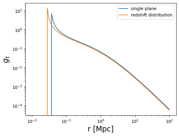
gt = m.compute_reduced_tangential_shear(
    r3d,
    mdelta=cluster_mass,
    cdelta=cluster_concentration,
    z_cluster=z_cl,
    z_src=z_src,
    cosmo=cosmo,
    delta_mdef=mass_Delta,
    halo_profile_model=density_profile_parametrization,
    z_src_info="discrete",
)
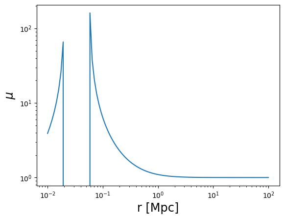
mu = m.compute_magnification(
    r3d,
    mdelta=cluster_mass,
    cdelta=cluster_concentration,
    z_cluster=z_cl,
    z_src=z_src,
    cosmo=cosmo,
    delta_mdef=mass_Delta,
    halo_profile_model=density_profile_parametrization,
    z_src_info="discrete",
)
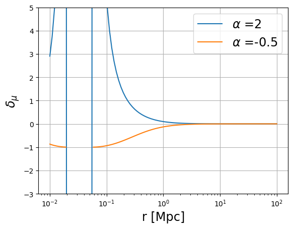
mu_bias = m.compute_magnification_bias(
    r3d,
    alpha=alpha,
    mdelta=cluster_mass,
    cdelta=cluster_concentration,
    z_cluster=z_cl,
    z_src=z_src,
    cosmo=cosmo,
    delta_mdef=mass_Delta,
    halo_profile_model=density_profile_parametrization,
    z_src_info="discrete",
)
/global/homes/a/aguena/.local/perlmutter/python-3.11/lib/python3.11/site-packages/clmm-1.12.0-py3.11.egg/clmm/theory/generic.py:66: UserWarning: Magnification is negative for certain radii,                     returning nan for magnification bias in this case.
/global/homes/a/aguena/.local/perlmutter/python-3.11/lib/python3.11/site-packages/clmm-1.12.0-py3.11.egg/clmm/theory/generic.py:70: RuntimeWarning: invalid value encountered in power
Lensing quantities assuming sources follow a given redshift distribution.
# Compute first beta
beta_kwargs = {
    "z_cl": z_cl,
    "z_inf": 10.0,
    "cosmo": cosmo,
    #'zmax' :zsrc_max,
    #'delta_z_cut': delta_z_cut,
    #'zmin': None,
    "z_distrib_func": z_distrib_func,
}
beta_s_mean = clmm.utils.compute_beta_s_mean_from_distribution(**beta_kwargs)
beta_s_square_mean = clmm.utils.compute_beta_s_square_mean_from_distribution(**beta_kwargs)

gt_z = m.compute_reduced_tangential_shear(
    r3d,
    mdelta=cluster_mass,
    cdelta=cluster_concentration,
    z_cluster=z_cl,
    z_src=[beta_s_mean, beta_s_square_mean],
    cosmo=cosmo,
    delta_mdef=mass_Delta,
    halo_profile_model=density_profile_parametrization,
    z_src_info="beta",
    approx="order2",
)
Plot the predicted profiles
def plot_profile(r, profile_vals, profile_label="rho", label=""):
    plt.loglog(r, profile_vals, label=label)
    plt.xlabel("r [Mpc]", fontsize="xx-large")
    plt.ylabel(profile_label, fontsize="xx-large")
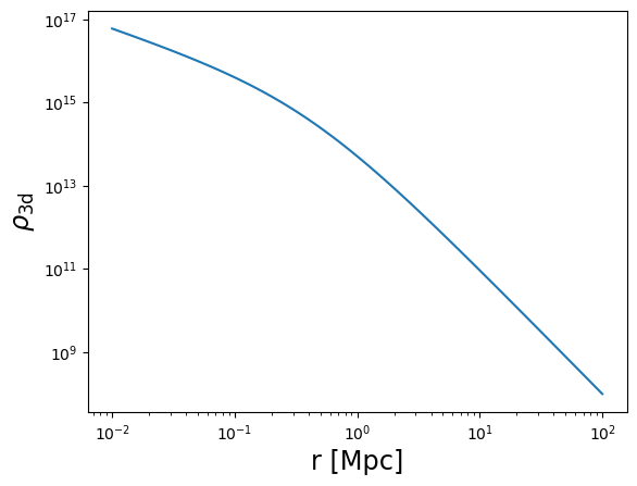
plot_profile(r3d, rho, "$\\rho_{\\rm 3d}$")
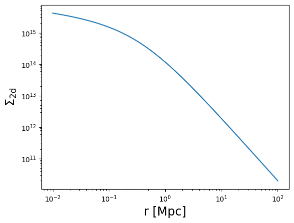
plot_profile(r3d, Sigma, "$\\Sigma_{\\rm 2d}$")
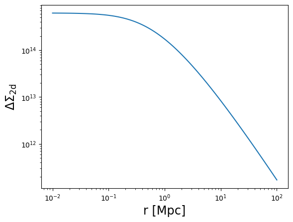
plot_profile(r3d, DeltaSigma, "$\\Delta\\Sigma_{\\rm 2d}$")
plot_profile(r3d, kappa, "$\\kappa$")
plot_profile(r3d, gammat, "$\\gamma_t$")
plot_profile(r3d, gt, "$g_t$", label="single plane")
plot_profile(r3d, gt_z, "$g_t$", label="redshift distribution")
plt.legend()
<matplotlib.legend.Legend at 0x7f8b21b8cbd0>
plot_profile(r3d, mu, "$\mu$")
plot_profile(
    r3d, mu_bias[0] - 1, profile_label="$\delta_{\mu}$", label="$\\alpha$ =" + str(alpha[0])
)
plot_profile(r3d, mu_bias[1] - 1, "$\delta_{\mu}$", label="$\\alpha$ =" + str(alpha[1]))

plt.legend(fontsize="xx-large")
plt.yscale("linear")
plt.grid()

plt.ylim(-3, 5)
(-3.0, 5.0)
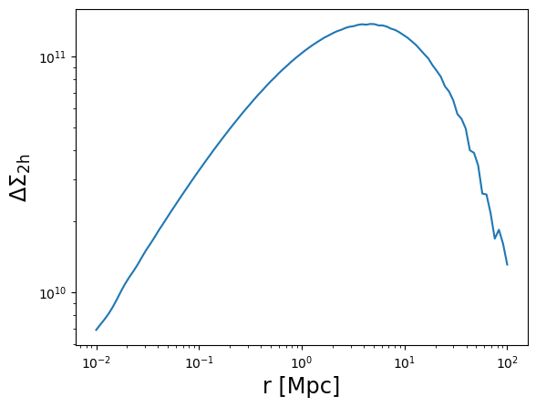
# The 2-halo term excess surface density is only implemented for the CCL and NC backends
# An error will be raised if using the CT backend instead

DeltaSigma_2h = m.compute_excess_surface_density_2h(r3d, z_cl, cosmo=cosmo, halobias=0.3)
plot_profile(r3d, DeltaSigma_2h, "$\\Delta\\Sigma_{\\rm 2h}$")
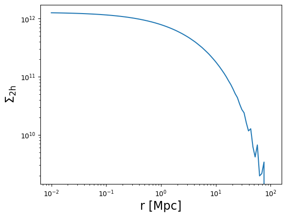
# The 2-halo term excess surface density is only implemented for the CCL and NC backends
# An error will be raised if using the CT backend instead

Sigma_2h = m.compute_surface_density_2h(r3d, z_cl, cosmo=cosmo, halobias=0.3)
plot_profile(r3d, Sigma_2h, "$\\Sigma_{\\rm 2h}$")
Side note regarding the Einasto profile (CCL and NC backends only)
The Einasto profile is supported by both the CCL and NumCosmo backends.
The value of the slope of the Einasto profile can be defined by the
user, using the alpha_ein keyword. If alpha_ein is not provided,
both backend revert to a default value for the Einasto slope: - In CCL,
the default Einasto slope depends on cosmology, redshift and halo mass.
- In NumCosmo, the default value is \(\alpha_{\rm ein}=0.25\).
NB: for CCL, setting a user-defined value for the Einasto slope is only available for versions >= 2.6. Earlier versions only allow the default option.
The verbose option allows to print the value of \(\alpha\) that is being used, as follows:
rho = m.compute_3d_density(
    r3d,
    mdelta=cluster_mass,
    cdelta=cluster_concentration,
    z_cl=z_cl,
    cosmo=cosmo,
    halo_profile_model="einasto",
    alpha_ein=0.17,
    verbose=True,
)

# For CCL < 2.6, the above call will return an error, as alpha_ein can not be set. The call below, not specifying alpha_ein,
# will use the default value (for both CCL and NC backends)

# rho = m.compute_3d_density(r3d, mdelta=cluster_mass, cdelta=cluster_concentration,
#                            z_cl=z_cl, cosmo=cosmo, halo_profile_model='einasto',
#                            verbose=True)


plot_profile(r3d, rho, "$\\rho_{\\rm 3d}$")
Einasto alpha = 0.17
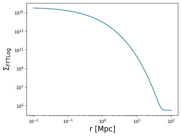
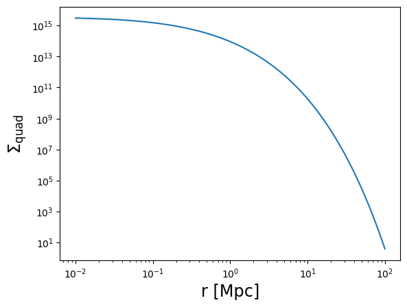
Side note regarding the Einasto profile (CCL backend only)
For CCL versions >= 2.8.1.dev73+g86125b08, the surface mass density
profile can be calculated with the quad_vec numerial integration in
addition to the default FFTLog. This option will increase the precision
of the profile at large radii and can be enabled by passing
use_projected_quad keyword argument to compute_surface_density.
# use quad_vec
Sigma_quad = m.compute_surface_density(
    r3d,
    mdelta=cluster_mass,
    cdelta=cluster_concentration,
    z_cl=z_cl,
    cosmo=cosmo,
    halo_profile_model="einasto",
    alpha_ein=0.17,
    use_projected_quad=True,  # use quad_vec
    verbose=True,
)

plot_profile(r3d, Sigma_quad, "$\\Sigma_{\\rm quad}$")
Einasto alpha = 0.3713561546989172
# default behavior
Sigma_FFTLog = m.compute_surface_density(
    r3d,
    mdelta=cluster_mass,
    cdelta=cluster_concentration,
    z_cl=z_cl,
    cosmo=cosmo,
    halo_profile_model="einasto",
    alpha_ein=0.17,
    use_projected_quad=False,  # default
    verbose=True,
)

plot_profile(r3d, Sigma_FFTLog, "$\\Sigma_{\\rm FFTLog}$")
Einasto alpha = 0.3713561546989172