Example 2: Realistic data and wrong model
Fit halo mass to shear profile with realistic data and wrong model
the LSST-DESC CLMM team
This notebook demonstrates how to use clmm to estimate a WL halo
mass from observations of a galaxy cluster. It uses several
functionalities of the support mock_data module to produce datasets
of increasing complexity. This notebook also demonstrates the bias
introduced on the reconstructed mass by a naive fit, when the redshift
distribution of the background galaxies is not properly accounted for in
the model. Organization of this notebook goes as follows:
Setting things up, with the proper imports.
Generating 3 datasets: an ideal dataset (dataset1) similar to that of Example1 (single source plane); an ideal dataset but with source galaxies following the Chang et al. (2013) redshift distribution (dataset2); a noisy dataset where photoz errors and shape noise are also included (dataset3).
Computing the binned reduced tangential shear profile, for the 3 datasets, using logarithmic binning.
Setting up the “single source plane” model to be fitted to the 3 datasets. Only dataset1 has a single source plane, so we expect to see a bias in the reconstructed mass when using this model on datasets 2 and 3.
Perform a simple fit using
scipy.optimize.curve_fitand visualize the results.
Setup
First, we import some standard packages.
import clmm
import matplotlib.pyplot as plt
import numpy as np
from numpy import random
from clmm.support.sampler import fitters

clmm.__version__
'1.12.0'
Next, we import clmm’s core modules.
import clmm.dataops as da
import clmm.galaxycluster as gc
import clmm.theory as theory
from clmm import Cosmology
We then import a support modules for a specific data sets. clmm
includes support modules that enable the user to generate mock data in a
format compatible with clmm.
from clmm.support import mock_data as mock
Making mock data
For reproducibility:
np.random.seed(11)
To create mock data, we need to define a true cosmology.
mock_cosmo = Cosmology(H0=70.0, Omega_dm0=0.27 - 0.045, Omega_b0=0.045, Omega_k0=0.0)
We now set some parameters for a mock galaxy cluster.
cosmo = mock_cosmo
cluster_m = 1.0e15  # M200,m [Msun]
cluster_z = 0.3
concentration = 4
ngals = 10000
Delta = 200
cluster_ra = 20.0
cluster_dec = 70.0
Then we use the mock_data support module to generate 3 galaxy
catalogs: - ideal_data: all background galaxies at the same
redshift. - ideal_data_z: galaxies distributed according to the
Chang et al. (2013) redshift distribution. - noisy_data_z:
ideal_data_z + photoz errors + shape noise
ideal_data = mock.generate_galaxy_catalog(
    cluster_m,
    cluster_z,
    concentration,
    cosmo,
    0.8,
    ngals=ngals,
    cluster_ra=cluster_ra,
    cluster_dec=cluster_dec,
)
ideal_data_z = mock.generate_galaxy_catalog(
    cluster_m,
    cluster_z,
    concentration,
    cosmo,
    "chang13",
    ngals=ngals,
    cluster_ra=cluster_ra,
    cluster_dec=cluster_dec,
)
noisy_data_z = mock.generate_galaxy_catalog(
    cluster_m,
    cluster_z,
    concentration,
    cosmo,
    "chang13",
    shapenoise=0.05,
    photoz_sigma_unscaled=0.05,
    ngals=ngals,
    cluster_ra=cluster_ra,
    cluster_dec=cluster_dec,
)
The galaxy catalogs are converted to a clmm.GalaxyCluster object and
may be saved for later use.
cluster_id = "CL_ideal"
gc_object = clmm.GalaxyCluster(cluster_id, cluster_ra, cluster_dec, cluster_z, ideal_data)
gc_object.save("ideal_GC.pkl")

cluster_id = "CL_ideal_z"
gc_object = clmm.GalaxyCluster(cluster_id, cluster_ra, cluster_dec, cluster_z, ideal_data_z)
gc_object.save("ideal_GC_z.pkl")

cluster_id = "CL_noisy_z"
gc_object = clmm.GalaxyCluster(cluster_id, cluster_ra, cluster_dec, cluster_z, noisy_data_z)
gc_object.save("noisy_GC_z.pkl")
Any saved clmm.GalaxyCluster object may be read in for analysis.
cl1 = clmm.GalaxyCluster.load("ideal_GC.pkl")  # all background galaxies at the same redshift
cl2 = clmm.GalaxyCluster.load(
    "ideal_GC_z.pkl"
)  # background galaxies distributed according to Chang et al. (2013)
cl3 = clmm.GalaxyCluster.load("noisy_GC_z.pkl")  # same as cl2 but with photoz error and shape noise

print("Cluster info = ID:", cl2.unique_id, "; ra:", cl2.ra, "; dec:", cl2.dec, "; z_l :", cl2.z)
print("The number of source galaxies is :", len(cl2.galcat))
Cluster info = ID: CL_ideal_z ; ra: 20.0 ; dec: 70.0 ; z_l : 0.3
The number of source galaxies is : 10000
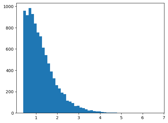
h = plt.hist(cl2.galcat["z"], bins=50)
Deriving observables
Computing shear
clmm.dataops.compute_tangential_and_cross_components calculates the
tangential and cross shears for each source galaxy in the cluster.
theta1, g_t1, g_x1 = cl1.compute_tangential_and_cross_components()
theta2, g_t2, g_x2 = cl2.compute_tangential_and_cross_components()
theta2, g_t3, g_x3 = cl3.compute_tangential_and_cross_components()
Radially binning the data
bin_edges = da.make_bins(0.7, 4, 15, method="evenlog10width")
clmm.dataops.make_radial_profile evaluates the average shear of the
galaxy catalog in bins of radius.
profile1 = cl1.make_radial_profile("Mpc", bins=bin_edges, cosmo=cosmo)
profile2 = cl2.make_radial_profile("Mpc", bins=bin_edges, cosmo=cosmo)
profile3 = cl3.make_radial_profile("Mpc", bins=bin_edges, cosmo=cosmo)
/global/homes/a/aguena/.local/perlmutter/python-3.11/lib/python3.11/site-packages/clmm-1.12.0-py3.11.egg/clmm/utils/statistic.py:97: RuntimeWarning: invalid value encountered in sqrt
After running clmm.dataops.make_radial_profile on a
clmm.GalaxyCluster object, the object acquires the
clmm.GalaxyCluster.profile attribute.
for n in cl1.profile.colnames:
    cl1.profile[n].format = "%6.3e"
cl1.profile.pprint(max_width=-1)
radius_min   radius  radius_max     gt      gt_err      gx       gx_err      z       z_err     n_src      W_l
---------- --------- ---------- --------- --------- ---------- --------- --------- --------- --------- ---------
 7.000e-01 7.446e-01  7.863e-01 4.359e-02 1.313e-04 -1.791e-17 1.058e-18 8.000e-01       nan 5.800e+01 5.800e+01
 7.863e-01 8.403e-01  8.831e-01 3.990e-02 1.101e-04 -1.573e-17 9.259e-19 8.000e-01 6.427e-09 8.600e+01 8.600e+01
 8.831e-01 9.395e-01  9.920e-01 3.659e-02 1.003e-04 -1.245e-17 8.502e-19 8.000e-01       nan 9.500e+01 9.500e+01
 9.920e-01 1.052e+00  1.114e+00 3.337e-02 8.507e-05 -1.269e-17 6.310e-19 8.000e-01       nan 1.320e+02 1.320e+02
 1.114e+00 1.187e+00  1.251e+00 3.007e-02 7.161e-05 -1.018e-17 5.609e-19 8.000e-01 3.321e-09 1.510e+02 1.510e+02
 1.251e+00 1.331e+00  1.406e+00 2.711e-02 6.612e-05 -1.023e-17 4.313e-19 8.000e-01       nan 1.670e+02 1.670e+02
 1.406e+00 1.495e+00  1.579e+00 2.428e-02 5.252e-05 -8.955e-18 3.321e-19 8.000e-01 3.367e-09 2.350e+02 2.350e+02
 1.579e+00 1.677e+00  1.773e+00 2.167e-02 3.915e-05 -8.762e-18 2.340e-19 8.000e-01       nan 3.430e+02 3.430e+02
 1.773e+00 1.887e+00  1.992e+00 1.918e-02 3.437e-05 -6.828e-18 2.168e-19 8.000e-01       nan 4.010e+02 4.010e+02
 1.992e+00 2.119e+00  2.237e+00 1.694e-02 2.755e-05 -6.239e-18 1.655e-19 8.000e-01 4.245e-09 4.990e+02 4.990e+02
 2.237e+00 2.377e+00  2.513e+00 1.490e-02 2.161e-05 -5.460e-18 1.265e-19 8.000e-01 4.009e-09 6.630e+02 6.630e+02
 2.513e+00 2.672e+00  2.823e+00 1.302e-02 1.846e-05 -4.757e-18 1.027e-19 8.000e-01       nan 7.800e+02 7.800e+02
 2.823e+00 2.999e+00  3.171e+00 1.136e-02 1.422e-05 -4.126e-18 7.797e-20 8.000e-01       nan 1.042e+03 1.042e+03
 3.171e+00 3.369e+00  3.561e+00 9.847e-03 1.131e-05 -3.659e-18 5.939e-20 8.000e-01 6.299e-09 1.301e+03 1.301e+03
 3.561e+00 3.781e+00  4.000e+00 8.514e-03 8.968e-06 -3.057e-18 4.728e-20 8.000e-01 4.246e-09 1.644e+03 1.644e+03
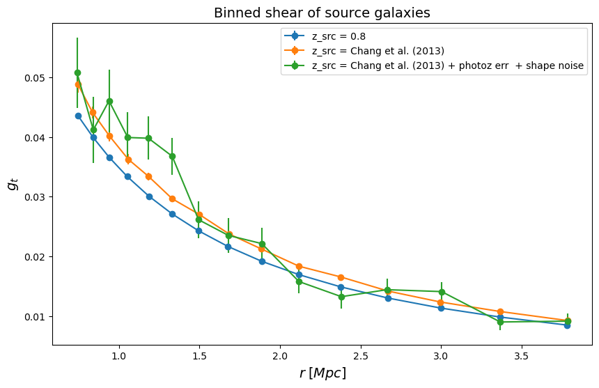
We visualize the radially binned shear for the 3 configurations
fig = plt.figure(figsize=(10, 6))


fsize = 14
fig.gca().errorbar(
    profile1["radius"], profile1["gt"], yerr=profile1["gt_err"], marker="o", label="z_src = 0.8"
)
fig.gca().errorbar(
    profile2["radius"],
    profile2["gt"],
    yerr=profile2["gt_err"],
    marker="o",
    label="z_src = Chang et al. (2013)",
)
fig.gca().errorbar(
    profile3["radius"],
    profile3["gt"],
    yerr=profile3["gt_err"],
    marker="o",
    label="z_src = Chang et al. (2013) + photoz err  + shape noise",
)

plt.gca().set_title(r"Binned shear of source galaxies", fontsize=fsize)
plt.gca().set_xlabel(r"$r\;[Mpc]$", fontsize=fsize)
plt.gca().set_ylabel(r"$g_t$", fontsize=fsize)
plt.legend()
<matplotlib.legend.Legend at 0x7f8080861b90>
Create the halo model
# model definition to be used with scipy.optimize.curve_fit
def shear_profile_model(r, logm, z_src):
    m = 10.0**logm
    gt_model = clmm.compute_reduced_tangential_shear(
        r, m, concentration, cluster_z, z_src, cosmo, delta_mdef=200, halo_profile_model="nfw"
    )
    return gt_model
Fitting a halo mass - highlighting bias when not accounting for the source redshift distribution in the model
We estimate the best-fit mass using scipy.optimize.curve_fit.
Here, to build the model we make the WRONG assumption that the average
shear in bin \(i\) equals the shear at the average redshift in the
bin; i.e. we assume that
\(\langle g_t\rangle_i = g_t(\langle z\rangle_i)\). This should not
impact cluster 1 as all sources are located at the same redshift.
However, this yields a bias in the reconstructed mass for cluster 2
and cluster 3, where the sources followed the Chang et al. (2013)
distribution.
# Cluster 1:  ideal data
popt1, pcov1 = fitters["curve_fit"](
    lambda r, logm: shear_profile_model(r, logm, profile1["z"]),
    profile1["radius"],
    profile1["gt"],
    profile1["gt_err"],
    bounds=[13.0, 17.0],
)
# popt1,pcov1 = spo.curve_fit(lambda r, logm:shear_profile_model(r, logm, profile1['z']),
#                    profile1['radius'],
#                    profile1['gt'],
#                    sigma=profile1['gt_err'], bounds=[13.,17.])

m_est1 = 10.0 ** popt1[0]
m_est_err1 = m_est1 * np.sqrt(pcov1[0][0]) * np.log(10)  # convert the error on logm to error on m

# Cluster 2:  ideal data with redshift distribution
popt2, pcov2 = fitters["curve_fit"](
    lambda r, logm: shear_profile_model(r, logm, profile2["z"]),
    profile2["radius"],
    profile2["gt"],
    profile2["gt_err"],
    bounds=[13.0, 17.0],
)

m_est2 = 10.0 ** popt2[0]
m_est_err2 = m_est2 * np.sqrt(pcov2[0][0]) * np.log(10)  # convert the error on logm to error on m

# Cluster 3:  noisy data with redshift distribution
popt3, pcov3 = fitters["curve_fit"](
    lambda r, logm: shear_profile_model(r, logm, profile3["z"]),
    profile3["radius"],
    profile3["gt"],
    profile3["gt_err"],
    bounds=[13.0, 17.0],
)

m_est3 = 10.0 ** popt3[0]
m_est_err3 = m_est3 * np.sqrt(pcov3[0][0]) * np.log(10)  # convert the error on logm to error on m


print(f"Best fit mass for cluster 1 = {m_est1:.2e} +/- {m_est_err1:.2e} Msun")
print(f"Best fit mass for cluster 2 = {m_est2:.2e} +/- {m_est_err2:.2e} Msun")
print(f"Best fit mass for cluster 3 = {m_est3:.2e} +/- {m_est_err3:.2e} Msun")
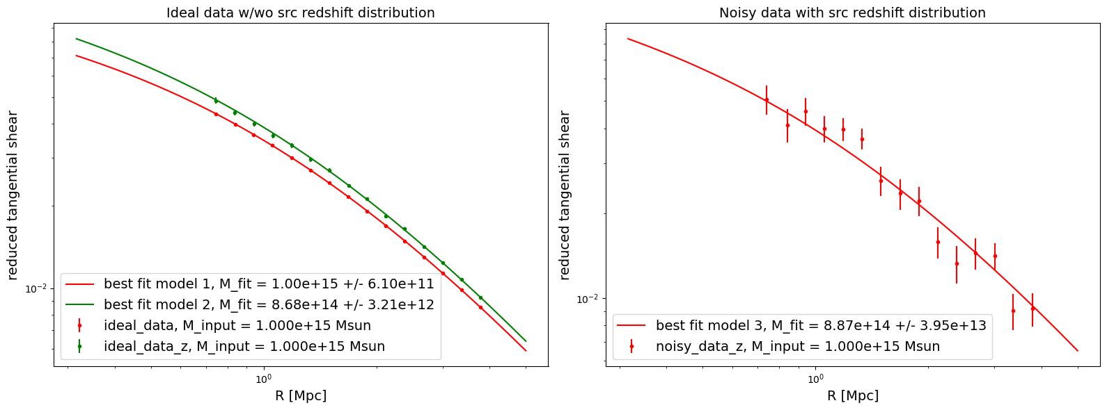
Best fit mass for cluster 1 = 1.00e+15 +/- 6.10e+11 Msun
Best fit mass for cluster 2 = 8.68e+14 +/- 3.21e+12 Msun
Best fit mass for cluster 3 = 8.87e+14 +/- 3.95e+13 Msun
As expected, the reconstructed mass is biased whenever the sources are not located at a single redshift as this was not accounted for in the model.
Visualization of the results
For visualization purpose, we calculate the reduced tangential shear predicted by the model when using the average redshift of the catalog.
rr = np.logspace(-0.5, np.log10(5), 100)
gt_model1 = clmm.compute_reduced_tangential_shear(
    rr,
    m_est1,
    concentration,
    cluster_z,
    np.mean(cl1.galcat["z"]),
    cosmo,
    delta_mdef=200,
    halo_profile_model="nfw",
)

gt_model2 = clmm.compute_reduced_tangential_shear(
    rr,
    m_est2,
    concentration,
    cluster_z,
    np.mean(cl2.galcat["z"]),
    cosmo,
    delta_mdef=200,
    halo_profile_model="nfw",
)

gt_model3 = clmm.compute_reduced_tangential_shear(
    rr,
    m_est3,
    concentration,
    cluster_z,
    np.mean(cl3.galcat["z"]),
    cosmo,
    delta_mdef=200,
    halo_profile_model="nfw",
)
We visualize that prediction of reduced tangential shear along with the data
fig, axes = plt.subplots(nrows=1, ncols=2, figsize=(16, 6))

axes[0].errorbar(
    profile1["radius"],
    profile1["gt"],
    profile1["gt_err"],
    color="red",
    label="ideal_data, M_input = %.3e Msun" % cluster_m,
    fmt=".",
)
axes[0].plot(
    rr,
    gt_model1,
    color="red",
    label="best fit model 1, M_fit = %.2e +/- %.2e" % (m_est1, m_est_err1),
)


axes[0].errorbar(
    profile2["radius"],
    profile2["gt"],
    profile2["gt_err"],
    color="green",
    label="ideal_data_z, M_input = %.3e Msun" % cluster_m,
    fmt=".",
)
axes[0].plot(
    rr,
    gt_model2,
    color="green",
    label="best fit model 2, M_fit = %.2e +/- %.2e" % (m_est2, m_est_err2),
)
axes[0].set_title("Ideal data w/wo src redshift distribution", fontsize=fsize)
axes[0].semilogx()
axes[0].semilogy()
axes[0].legend(fontsize=fsize)
axes[0].set_xlabel("R [Mpc]", fontsize=fsize)
axes[0].set_ylabel("reduced tangential shear", fontsize=fsize)

axes[1].errorbar(
    profile3["radius"],
    profile3["gt"],
    profile3["gt_err"],
    color="red",
    label="noisy_data_z, M_input = %.3e Msun" % cluster_m,
    fmt=".",
)
axes[1].plot(
    rr,
    gt_model3,
    color="red",
    label="best fit model 3, M_fit = %.2e +/- %.2e" % (m_est3, m_est_err3),
)
axes[1].set_title("Noisy data with src redshift distribution", fontsize=fsize)
axes[1].semilogx()
axes[1].semilogy()
axes[1].legend(fontsize=fsize)
axes[1].set_xlabel("R [Mpc]", fontsize=fsize)
axes[1].set_ylabel("reduced tangential shear", fontsize=fsize)

fig.tight_layout()