Example 4: Using a real dataset (HSC)

Fit halo mass to shear profile using HSC data

the LSST-DESC CLMM team

This notebook can be run on NERSC.

Here we demonstrate how to run CLMM on real observational datasets. As an example, we use the data from the Hyper Suprime-Cam Subaru Strategic Program (HSC SSP) public releases (Aihara+2018ab, 2019; Mandelbaum+2018ab) (Credit: NAOJ / HSC Collaboration), which have similar observation conditions and data formats to the Rubin LSST.

The steps in this notebook includes: - Setting things up - Selecting a cluster - Downloading the published catalog at the cluster field - Loading the catalog into CLMM - Running CLMM on the dataset

Links:

The data access of the HSC SSP Public Data Release: https://hsc-release.mtk.nao.ac.jp/doc/index.php/data-access__pdr3/

Shape catalog: https://hsc-release.mtk.nao.ac.jp/doc/index.php/s16a-shape-catalog-pdr2/

FAQ: https://hsc-release.mtk.nao.ac.jp/doc/index.php/faq__pdr3/

Photometric redshifts: https://hsc-release.mtk.nao.ac.jp/doc/index.php/photometric-redshifts/

Cluster catalog: https://hsc-release.mtk.nao.ac.jp/doc/index.php/camira_pdr2/

## 1. Setup

We import packages.

import numpy as np
import matplotlib.pyplot as plt

# %matplotlib inline
from astropy.table import Table
import pickle as pkl
from pathlib import Path

## 2. Selecting a cluster

We use the HSC SSP publications (https://hsc.mtk.nao.ac.jp/ssp/publications/) to select a list of reported massive galaxy clusters that have been measured by weak lensing. In the table below, the coordinates are for lensing peaks unless otherwise specified, and we assume h=0.7.

Name		RA (deg)	DEC (deg)	WL Mass	Re ference	Note
HWL 16a-094	0.592	2 23.0801	0.1689	15.3, 7.8	Ha mana+20 20	CAMIRA ID 1417; Miyaza ki+2018 rank 34
HWL 16a-026	0.424	1 30.5895	1.6473	8.7, 4.7	Ha mana+20 20	–
HWL 16a-034	0.315	1 39.0387	−0.3966	8.1, 5.6	Ha mana+20 20	Abell 776; MACS J0916. 1−0023; Miyaza ki+2018 rank 8; see also M edezins ki+2018
Rank 9	0.312	37.3951	−3.6099	–, 5.9	Miya zaki+20 18	–
Rank 48	0.529	2 20.7900	1.0509	–, 10.4	Miya zaki+20 18	–
Rank 62	0.592	2 16.6510	0.7982	–, 10.2	Miya zaki+20 18	–
MaxBCG J140. 53188+0 3.76632	0.2701	14 0.54565	3.77820	44.3, 25.1	Me dezinsk i+2018	BCG center (close to the X-ray c enter); PSZ2 G228.50 +34.95; double BCGs
X LSSC006	0.429	35.439	−3.772	9.6, 5.6	Um etsu+20 20	X-ray center

## 3. Downloading the catalog at the cluster field

The 3 most massive cluster-candidates are MaxBCG.J140.53188+03.76632 (in the GAMA09H field), Miyazaki+2018 (M18 hearafter) rank 48 and 62 (in the GAMA15H field). We consider MaxBCG.J140.53188+03.76632 first. The webpage for HSC SSP data access is here link. To download the catalogs, we need to first register for a user account (link). Then we log into the system, query and download the catalogs at CAS Search; we use object_id to cross match the shape catalog, photo-z catalog, and photometry catalog. Since the clusters are at redshift about 0.4, a radius of 10 arcmin would be about 3 Mpc. However, we make a query for the whole field to save time. The final catalog includes shape info, photo-z, and photometry. Here is an example of the query SQL command (thank Calum Murray; example command; schema); the query could take 1 hour and the size of the catalog could be 400 MB (.csv.gz). If you would like to test it, please copy from “select” to “–LIMIT 5”. Also select “PDR1” or press “Guess release from your SQL” at the CAS Search webpage. To unpress the file “.gz”, use “gunzip” or “gzip -d”.

select
 b.*,
 c.ira, c.idec,
 a.ishape_hsm_regauss_e1, a.ishape_hsm_regauss_e2,
 a.ishape_hsm_regauss_resolution, a.ishape_hsm_regauss_sigma,
 d1.photoz_best as ephor_ab_photoz_best, d1.photoz_risk_best as ephor_ab_photoz_risk_best,
 d2.photoz_best as frankenz_photoz_best, d2.photoz_risk_best as frankenz_photoz_risk_best,
 d3.photoz_best as nnpz_photoz_best, d3.photoz_risk_best as nnpz_photoz_risk_best,
 e.icmodel_mag, e.icmodel_mag_err,
 e.detect_is_primary,
 e.iclassification_extendedness,
 e.icmodel_flux_flags,
 e.icmodel_flux, e.icmodel_flux_err,
 c.iblendedness_abs_flux
from
 s16a_wide.meas2 a
 inner join s16a_wide.weaklensing_hsm_regauss b using (object_id)
 inner join s16a_wide.meas c using (object_id)
 -- inner join s16a_wide.photoz_demp d using (object_id)
 -- inner join s16a_wide.photoz_ephor d using (object_id)
  inner join s16a_wide.photoz_ephor_ab d1 using (object_id)
  inner join s16a_wide.photoz_frankenz d2 using (object_id)
 -- inner join s16a_wide.photoz_mizuki d using (object_id)
 -- inner join s16a_wide.photoz_mlz d using (object_id)
  inner join s16a_wide.photoz_nnpz d3 using (object_id)
  inner join s16a_wide.forced e using (object_id)
-- Uncomment the specific lines depending upon the field to be used
 -- where s16a_wide.search_xmm(c.skymap_id)
 -- where s16a_wide.search_wide01h(c.skymap_id)
 -- where s16a_wide.search_vvds(c.skymap_id)
 -- where s16a_wide.search_hectomap(c.skymap_id)
 -- where s16a_wide.search_gama15h(c.skymap_id)
 where s16a_wide.search_gama09h(c.skymap_id)
 --AND e.detect_is_primary
 --AND conesearch(c.icoord, 140.54565, 3.77820, 600)
 --AND NOT e.icmodel_flux_flags
 --AND e.iclassification_extendedness>0.5
 --LIMIT 5

## 4. Loading the catalog into CLMM

Once we have the catalog, we read in the catalog, make cuts on the catalog, and adjust column names to prepare for the analysis in CLMM.

%%time
# Assume the downloaded catalog is at this path:
filename = "197376_GAMMA09H.csv"
catalog = filename.replace(".csv", ".pkl")
if not Path(catalog).is_file():
    data_0 = Table.read(filename, format="ascii.csv")
    pkl.dump(data_0, open(catalog, "wb"))
else:
    data_0 = pkl.load(open(catalog, "rb"))

CPU times: user 141 ms, sys: 738 ms, total: 879 ms
Wall time: 886 ms

print(data_0.colnames)

['# object_id', 'ishape_hsm_regauss_derived_shape_weight', 'ishape_hsm_regauss_derived_shear_bias_m', 'ishape_hsm_regauss_derived_shear_bias_c1', 'ishape_hsm_regauss_derived_shear_bias_c2', 'ishape_hsm_regauss_derived_sigma_e', 'ishape_hsm_regauss_derived_rms_e', 'ira', 'idec', 'ishape_hsm_regauss_e1', 'ishape_hsm_regauss_e2', 'ishape_hsm_regauss_resolution', 'ishape_hsm_regauss_sigma', 'ephor_ab_photoz_best', 'ephor_ab_photoz_risk_best', 'frankenz_photoz_best', 'frankenz_photoz_risk_best', 'nnpz_photoz_best', 'nnpz_photoz_risk_best', 'icmodel_mag', 'icmodel_mag_err', 'detect_is_primary', 'iclassification_extendedness', 'icmodel_flux_flags', 'icmodel_flux', 'icmodel_flux_err', 'iblendedness_abs_flux']

# We select "frankenz" for the test, but there are other methods available.
photoz_type = "frankenz"
# photoz_type = "nnpz"
# photoz_type = "ephor_ab"

# Cuts
def make_cuts(catalog_in):
    # We consider some cuts in Mandelbaum et al. 2018 (HSC SSP Y1 shear catalog).
    select = catalog_in["detect_is_primary"] == "True"
    select &= catalog_in["icmodel_flux_flags"] == "False"
    select &= catalog_in["iclassification_extendedness"] > 0.5
    select &= catalog_in["icmodel_mag_err"] <= 2.5 / np.log(10.0) / 10.0
    select &= (
        catalog_in["ishape_hsm_regauss_e1"] ** 2 + catalog_in["ishape_hsm_regauss_e2"] ** 2 < 4.0
    )
    select &= catalog_in["icmodel_mag"] <= 24.5
    select &= catalog_in["iblendedness_abs_flux"] < (10 ** (-0.375))
    select &= catalog_in["ishape_hsm_regauss_resolution"] >= 0.3  # similar to extendedness
    select &= catalog_in["ishape_hsm_regauss_sigma"] <= 0.4
    # Note "zbest" minimizes the risk of the photo-z point estimate being far away from the true value.
    # Details: https://hsc-release.mtk.nao.ac.jp/doc/wp-content/uploads/2017/02/pdr1_photoz_release_note.pdf
    select &= catalog_in["%s_photoz_risk_best" % photoz_type] < 0.5

    catalog_out = catalog_in[select]

    return catalog_out


data_1 = make_cuts(data_0)
print(len(data_0), len(data_1), len(data_1) * 1.0 / len(data_0))

2678766 2514470 0.9386672818753112

# Reference: Mandelbaum et al. 2018 "The first-year shear catalog of the Subaru Hyper Suprime-Cam Subaru Strategic Program Survey".
# Section A.3.2: "per-object galaxy shear estimate".
def apply_shear_calibration(catalog_in):
    e1_0 = catalog_in["ishape_hsm_regauss_e1"]
    e2_0 = catalog_in["ishape_hsm_regauss_e2"]
    e_rms = catalog_in["ishape_hsm_regauss_derived_rms_e"]
    m = catalog_in["ishape_hsm_regauss_derived_shear_bias_m"]
    c1 = catalog_in["ishape_hsm_regauss_derived_shear_bias_c1"]
    c2 = catalog_in["ishape_hsm_regauss_derived_shear_bias_c2"]
    # Note: in the mass fit we have not implemented the weight yet.
    weight = catalog_in["ishape_hsm_regauss_derived_shape_weight"]

    R = 1.0 - np.sum(weight * e_rms**2.0) / np.sum(weight)
    m_mean = np.sum(weight * m) / np.sum(weight)
    c1_mean = np.sum(weight * c1) / np.sum(weight)
    c2_mean = np.sum(weight * c2) / np.sum(weight)
    print("R, m_mean, c1_mean, c2_mean: ", R, m_mean, c1_mean, c2_mean)

    g1 = (e1_0 / (2.0 * R) - c1) / (1.0 + m_mean)
    g2 = (e2_0 / (2.0 * R) - c2) / (1.0 + m_mean)

    return g1, g2

# Adjust column names.
def adjust_column_names(catalog_in):
    # We consider a map between new and old column names.
    # Note we have considered shear calibration here.
    column_name_map = {
        "ra": "ira",
        "dec": "idec",
        "z": "%s_photoz_best" % photoz_type,
        "id": "# object_id",
    }

    catalog_out = Table()
    for i in column_name_map:
        catalog_out[i] = catalog_in[column_name_map[i]]

    g1, g2 = apply_shear_calibration(catalog_in)
    # CLMM uses "epsilon shape" rather than "chi shape".
    catalog_out["e1"] = g1
    catalog_out["e2"] = g2

    return catalog_out


data_2 = adjust_column_names(data_1)

R, m_mean, c1_mean, c2_mean:  0.840031677829739 -0.10973213380132621 -0.0001494161260923776 1.7902495719644782e-05

# Make some figures for visualization.
def make_plots(catalog_in):
    # Scatter plot
    plt.figure()
    plt.scatter(catalog_in["ra"], catalog_in["dec"], c=catalog_in["z"], s=1.0, alpha=0.2)
    plt.colorbar()
    plt.xlabel("ra")
    plt.ylabel("dec")
    plt.title("z")

    # Histogram
    plt.figure()
    plt.hist(catalog_in["z"], bins=20)
    plt.xlabel("z")
    plt.ylabel("count")

    # Relation
    plt.figure()
    plt.plot(catalog_in["e1"], catalog_in["e2"], ",")
    plt.xlabel("e1")
    plt.ylabel("e2")


# make_plots(data_2)

## 5. Running CLMM on the dataset We use the functions similar to examples/Paper_v1.0/gt_and_use_case.ipynb.

from clmm import Cosmology

cosmo = Cosmology(H0=70.0, Omega_dm0=0.27 - 0.045, Omega_b0=0.045, Omega_k0=0.0)

# We consider MaxBCG J140.53188+03.76632
cluster_z = 0.2701  # Cluster redshift
cluster_ra = 140.54565  # Cluster Ra in deg
cluster_dec = 3.77820  # Cluster Dec in deg

obs_galaxies = data_2

obs_galaxies = obs_galaxies[(obs_galaxies["z"] > (cluster_z + 0.1))]

# Area cut: the query is made for the whole field and this can simplify the processing.
select = obs_galaxies["ra"] < cluster_ra + 12.0 / 60.0 / np.cos(cluster_dec / 180.0 * np.pi)
select &= obs_galaxies["ra"] > cluster_ra - 12.0 / 60.0 / np.cos(cluster_dec / 180.0 * np.pi)
select &= obs_galaxies["dec"] < cluster_dec + 12.0 / 60.0
select &= obs_galaxies["dec"] > cluster_dec - 12.0 / 60.0
obs_galaxies = obs_galaxies[select]

obs_galaxies["id"] = np.arange(len(obs_galaxies))

# Put galaxy values on arrays.
gal_ra = obs_galaxies["ra"]  # Galaxies Ra in deg
gal_dec = obs_galaxies["dec"]  # Galaxies Dec in deg
gal_e1 = obs_galaxies["e1"]  # Galaxies elipticipy 1
gal_e2 = obs_galaxies["e2"]  # Galaxies elipticipy 2
gal_z = obs_galaxies["z"]  # Galaxies observed redshift
gal_id = obs_galaxies["id"]  # Galaxies ID

# Using the GalaxyCluster object.

import clmm
import clmm.dataops as da
from clmm.utils import convert_units

# Create a GCData with the galaxies.
galaxies = clmm.GCData(
    [gal_ra, gal_dec, gal_e1, gal_e2, gal_z, gal_id], names=["ra", "dec", "e1", "e2", "z", "id"]
)

# Create a GalaxyCluster.
cluster = clmm.GalaxyCluster("Name of cluster", cluster_ra, cluster_dec, cluster_z, galaxies)

# Convert elipticities into shears for the members.
cluster.compute_tangential_and_cross_components()
print(cluster.galcat.colnames)

# Measure profile and add profile table to the cluster.
seps = convert_units(cluster.galcat["theta"], "radians", "Mpc", cluster.z, cosmo)

cluster.make_radial_profile(
    bins=da.make_bins(0.3, 3.0, 15, method="evenlog10width"),
    bin_units="Mpc",
    cosmo=cosmo,
    include_empty_bins=False,
    gal_ids_in_bins=True,
)
print(cluster.profile.colnames)

['ra', 'dec', 'e1', 'e2', 'z', 'id', 'theta', 'et', 'ex']
['radius_min', 'radius', 'radius_max', 'gt', 'gt_err', 'gx', 'gx_err', 'z', 'z_err', 'n_src', 'W_l', 'gal_id']

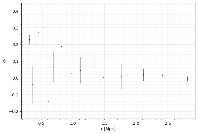
fig = plt.figure(figsize=(6, 4))
ax = fig.add_axes((0, 0, 1, 1))
errorbar_kwargs = dict(linestyle="", marker="o", markersize=1, elinewidth=0.5, capthick=0.5)
ax.errorbar(
    cluster.profile["radius"],
    cluster.profile["gt"],
    cluster.profile["gt_err"],
    c="k",
    **errorbar_kwargs
)
ax.set_xlabel("r [Mpc]", fontsize=10)
ax.set_ylabel(r"$g_t$", fontsize=10)
ax.grid(lw=0.3)
ax.minorticks_on()
ax.grid(which="minor", lw=0.1)
plt.show()

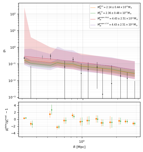
# Theoretical predictions

# Model relying on the overall redshift distribution of the sources (WtG III Applegate et al. 2014).
# Note the concentration of MaxBCG J140.53188+03.76632 was not reported.
# The value from the stacked sample in the paper is ~7.
# For the mass scale, a typical c-M relation (e.g. Child et al. 2018) would give c~3 though.
# And we have not considered a c-M relation in the fitting.
z_inf = 1000
concentration = 4.0

bs_mean = np.mean(clmm.utils.compute_beta_s(cluster.galcat["z"], cluster_z, z_inf, cosmo))
bs2_mean = np.mean(clmm.utils.compute_beta_s(cluster.galcat["z"], cluster_z, z_inf, cosmo) ** 2)


def predict_reduced_tangential_shear_redshift_distribution(profile, logm):
    gt = clmm.compute_reduced_tangential_shear(
        r_proj=profile["radius"],  # Radial component of the profile
        mdelta=10**logm,  # Mass of the cluster [M_sun]
        cdelta=concentration,  # Concentration of the cluster
        z_cluster=cluster_z,  # Redshift of the cluster
        z_src=(bs_mean, bs2_mean),  # tuple of (bs_mean, bs2_mean)
        z_src_info="beta",
        approx="order1",
        cosmo=cosmo,
        delta_mdef=200,
        massdef="critical",
        halo_profile_model="nfw",
    )
    return gt


# Model using individual redshift and radial information, to compute the averaged shear in each radial bin, based on the galaxies actually present in that bin.
cluster.galcat["theta_mpc"] = convert_units(
    cluster.galcat["theta"], "radians", "mpc", cluster.z, cosmo
)


def predict_reduced_tangential_shear_individual_redshift(profile, logm):
    return np.array(
        [
            np.mean(
                clmm.compute_reduced_tangential_shear(
                    # Radial component of each source galaxy inside the radial bin
                    r_proj=cluster.galcat[radial_bin["gal_id"]]["theta_mpc"],
                    mdelta=10**logm,  # Mass of the cluster [M_sun]
                    cdelta=concentration,  # Concentration of the cluster
                    z_cluster=cluster_z,  # Redshift of the cluster
                    # Redshift value of each source galaxy inside the radial bin
                    z_src=cluster.galcat[radial_bin["gal_id"]]["z"],
                    cosmo=cosmo,
                    delta_mdef=200,
                    massdef="critical",
                    halo_profile_model="nfw",
                )
            )
            for radial_bin in profile
        ]
    )

# Mass fitting

mask_for_fit = cluster.profile["n_src"] > 2
data_for_fit = cluster.profile[mask_for_fit]

from clmm.support.sampler import fitters


def fit_mass(predict_function):
    popt, pcov = fitters["curve_fit"](
        predict_function,
        data_for_fit,
        data_for_fit["gt"],
        data_for_fit["gt_err"],
        bounds=[10.0, 17.0],
    )
    logm, logm_err = popt[0], np.sqrt(pcov[0][0])
    return {
        "logm": logm,
        "logm_err": logm_err,
        "m": 10**logm,
        "m_err": (10**logm) * logm_err * np.log(10),
    }

# In the paper, the measured mass is 44.3 {+ 30.3} {- 19.9} * 10^14 Msun (M200c,WL).
# For convenience, we consider a mean value for the errorbar.
# We build a dictionary based on that result.
m_paper = 44.3e14
m_err_paper = 25.1e14
logm_paper = np.log10(m_paper)
logm_err_paper = m_err_paper / (10**logm_paper) / np.log(10)
paper_value = {
    "logm": logm_paper,
    "logm_err": logm_err_paper,
    "m": 10**logm_paper,
    "m_err": (10**logm_paper) * logm_err_paper * np.log(10),
}

%%time
fit_redshift_distribution = fit_mass(predict_reduced_tangential_shear_redshift_distribution)
fit_individual_redshift = fit_mass(predict_reduced_tangential_shear_individual_redshift)

CPU times: user 332 ms, sys: 2.91 ms, total: 335 ms
Wall time: 333 ms

print(
    f'Best fit mass for N(z) model                     = {fit_redshift_distribution["m"]:.3e} +/- {fit_redshift_distribution["m_err"]:.3e} Msun'
)
print(
    f'Best fit mass for individual redshift and radius = {fit_individual_redshift["m"]:.3e} +/- {fit_individual_redshift["m_err"]:.3e} Msun'
)

Best fit mass for N(z) model                     = 2.137e+15 +/- 4.397e+14 Msun
Best fit mass for individual redshift and radius = 2.358e+15 +/- 4.764e+14 Msun

# Visualization of the results.
def get_predicted_shear(predict_function, fit_values):
    gt_est = predict_function(data_for_fit, fit_values["logm"])
    gt_est_err = [
        predict_function(data_for_fit, fit_values["logm"] + i * fit_values["logm_err"])
        for i in (-3, 3)
    ]
    return gt_est, gt_est_err


gt_redshift_distribution, gt_err_redshift_distribution = get_predicted_shear(
    predict_reduced_tangential_shear_redshift_distribution, fit_redshift_distribution
)
gt_individual_redshift, gt_err_individual_redshift = get_predicted_shear(
    predict_reduced_tangential_shear_individual_redshift, fit_individual_redshift
)

gt_paper1, gt_err_paper1 = get_predicted_shear(
    predict_reduced_tangential_shear_redshift_distribution, paper_value
)
gt_paper2, gt_err_paper2 = get_predicted_shear(
    predict_reduced_tangential_shear_individual_redshift, paper_value
)

chi2_redshift_distribution_dof = np.sum(
    (gt_redshift_distribution - data_for_fit["gt"]) ** 2 / (data_for_fit["gt_err"]) ** 2
) / (len(data_for_fit) - 1)
chi2_individual_redshift_dof = np.sum(
    (gt_individual_redshift - data_for_fit["gt"]) ** 2 / (data_for_fit["gt_err"]) ** 2
) / (len(data_for_fit) - 1)

print(f"Reduced chi2 (N(z) model) = {chi2_redshift_distribution_dof}")
print(f"Reduced chi2 (individual (R,z) model) = {chi2_individual_redshift_dof}")

Reduced chi2 (N(z) model) = 2.4805403526932412
Reduced chi2 (individual (R,z) model) = 2.6209850216324857

from matplotlib.ticker import MultipleLocator

fig = plt.figure(figsize=(6, 6))
gt_ax = fig.add_axes((0.25, 0.42, 0.7, 0.55))
gt_ax.errorbar(
    data_for_fit["radius"], data_for_fit["gt"], data_for_fit["gt_err"], c="k", **errorbar_kwargs
)

# Points in grey have not been used for the fit.
gt_ax.errorbar(
    cluster.profile["radius"][~mask_for_fit],
    cluster.profile["gt"][~mask_for_fit],
    cluster.profile["gt_err"][~mask_for_fit],
    c="grey",
    **errorbar_kwargs,
)

pow10 = 15
mlabel = lambda name, fits: (
    rf"$M_{{fit}}^{{{name}}} = "
    rf'{fits["m"]/10**pow10:.2f}\pm'
    rf'{fits["m_err"]/10**pow10:.2f}'
    rf"\times 10^{{{pow10}}} M_\odot$"
)

# The model for the 1st method.
gt_ax.loglog(
    data_for_fit["radius"],
    gt_redshift_distribution,
    "-C1",
    label=mlabel("N(z)", fit_redshift_distribution),
    lw=0.5,
)
gt_ax.fill_between(
    data_for_fit["radius"], *gt_err_redshift_distribution, lw=0, color="C1", alpha=0.2
)

# The model for the 2nd method.
gt_ax.loglog(
    data_for_fit["radius"],
    gt_individual_redshift,
    "-C2",
    label=mlabel("z,R", fit_individual_redshift),
    lw=0.5,
)
gt_ax.fill_between(data_for_fit["radius"], *gt_err_individual_redshift, lw=0, color="C2", alpha=0.2)

# The value in the reference paper.
gt_ax.loglog(
    data_for_fit["radius"], gt_paper1, "-C3", label=mlabel("paper; N(z)", paper_value), lw=0.5
)
gt_ax.fill_between(data_for_fit["radius"], *gt_err_paper1, lw=0, color="C3", alpha=0.2)

gt_ax.loglog(
    data_for_fit["radius"], gt_paper2, "-C4", label=mlabel("paper; Z,R", paper_value), lw=0.5
)
gt_ax.fill_between(data_for_fit["radius"], *gt_err_paper2, lw=0, color="C4", alpha=0.2)

gt_ax.set_ylabel(r"$g_t$", fontsize=8)
gt_ax.legend(fontsize=6)
gt_ax.set_xticklabels([])
gt_ax.tick_params("x", labelsize=8)
gt_ax.tick_params("y", labelsize=8)


errorbar_kwargs2 = {k: v for k, v in errorbar_kwargs.items() if "marker" not in k}
errorbar_kwargs2["markersize"] = 3
errorbar_kwargs2["markeredgewidth"] = 0.5
res_ax = fig.add_axes((0.25, 0.2, 0.7, 0.2))
delta = (cluster.profile["radius"][1] / cluster.profile["radius"][0]) ** 0.25


res_ax.errorbar(
    data_for_fit["radius"],
    data_for_fit["gt"] / gt_redshift_distribution - 1,
    yerr=data_for_fit["gt_err"] / gt_redshift_distribution,
    marker="s",
    c="C1",
    **errorbar_kwargs2,
)
errorbar_kwargs2["markersize"] = 3
errorbar_kwargs2["markeredgewidth"] = 0.5

res_ax.errorbar(
    data_for_fit["radius"] * delta,
    data_for_fit["gt"] / gt_individual_redshift - 1,
    yerr=data_for_fit["gt_err"] / gt_individual_redshift,
    marker="*",
    c="C2",
    **errorbar_kwargs2,
)
res_ax.set_xlabel(r"$R$ [Mpc]", fontsize=8)

res_ax.set_ylabel(r"$g_t^{data}/g_t^{mod.}-1$", fontsize=8)
res_ax.set_xscale("log")

res_ax.set_ylim(-5, 5)
res_ax.yaxis.set_minor_locator(MultipleLocator(10))

res_ax.tick_params("x", labelsize=8)
res_ax.tick_params("y", labelsize=8)

for ax in (gt_ax, res_ax):
    ax.grid(lw=0.3)
    ax.minorticks_on()
    ax.grid(which="minor", lw=0.1)
plt.show()

Reference

Aihara, H., Arimoto, N., Armstrong, R., et al. 2018, Publications of the Astronomical Society of Japan, 70, S4

Aihara, H., Armstrong, R., Bickerton, S., et al. 2018, Publications of the Astronomical Society of Japan, 70, S8

Aihara, H., AlSayyad, Y., Ando, M., et al. 2019, Publications of the Astronomical Society of Japan, 71

Hamana, T., Shirasaki, M., Lin, Y.-T., 2020, Publications of the Astronomical Society of Japan, 72, 78

Mandelbaum, R., Miyatake, H., Hamana, T., et al. 2018, Publications of the Astronomical Society of Japan, 70, S25

Mandelbaum, R., Lanusse, F., Leauthaud, A., et al. 2018, Monthly Notices of the Royal Astronomical Society, 481, 3170

Medezinski, E., Battaglia, N., Umetsu, K., et al., 2018, Publications of the Astronomical Society of Japan, 70, S28

Miyazaki, S., Oguri, M., Hamana, T., et al., 2018, Publications of the Astronomical Society of Japan, 70, S27

Umetsu, K., Sereno, M., Lieu, M., et al., 2020, Astrophysical Journal, 890, 148