Generate “realistic” mock data for a cluster ensemble

Generate cluster ensemble with “realistic” mass and redshift distribution

In this notebook, we generate a ‘realistic’ mock cluster ensemble, i.e. given a halo mass function, and mass-concentration relation (more complexity, such as miscentering, could also be added but it’s not done here). The notebook is structured as follows: - Implementation of the CCL and NumCosmo mass functions. - Some comparisons between the different backends. - Implementation of a accept-reject method to generate cluster samples from the mass function. - Generation of a cluster catalog for mass and redshift bins followed by a comparison with the theoretical prediction

Then, the remaining of the notebook repeats what was done in the Example_cluster_ensemble.ipynb. - Geration of mock galaxy data for each cluster - Creating ClusterEnsemble object and estimation of individual excess surface density profiles - An analysis of the covariance of the stack between radial bins

Draw pairs of mass and redshift according to a mass function (computed with either CCL or NumCosmo)

In this notebook we use the Tinker halo mass function, and demonstrate the implementation via CCL or NumCosmo.

import sys
import numpy as np
import pyccl as ccl
import matplotlib.pyplot as plt
import scipy
import clmm
from clmm import GalaxyCluster, ClusterEnsemble, GCData
from clmm import Cosmology
from clmm.support import mock_data as mock

%matplotlib inline

# NumCosmo imports
try:
    import gi

    gi.require_version("NumCosmo", "1.0")
    gi.require_version("NumCosmoMath", "1.0")
except:
    pass

from gi.repository import GObject
from gi.repository import NumCosmo as Nc
from gi.repository import NumCosmoMath as Ncm

Ncm.cfg_init()
Ncm.cfg_set_log_handler(lambda msg: sys.stdout.write(msg) and sys.stdout.flush())

For reproducibility:

np.random.seed(11)

Mass function - CCL implementation

cosmo = ccl.Cosmology(
    Omega_c=0.26,
    Omega_b=0.04,
    h=0.7,
    sigma8=0.8,
    n_s=0.96,
    Neff=3.04,
    m_nu=1.0e-05,
    mass_split="single",
)
hmd_200c = ccl.halos.MassDef(200, "critical")


# For a different multiplicty function, the user must change this function below
def tinker08_ccl(logm, z):
    mass = 10 ** (logm)
    hmf_200c = ccl.halos.MassFuncTinker08(mass_def=hmd_200c)
    nm = hmf_200c(cosmo, mass, 1.0 / (1 + z))
    return nm  # dn/dlog10M


# Computing the volume element
def dV_over_dOmega_dz(z):
    a = 1.0 / (1.0 + z)
    da = ccl.background.angular_diameter_distance(cosmo, a)
    E = ccl.background.h_over_h0(cosmo, a)
    return ((1.0 + z) ** 2) * (da**2) * ccl.physical_constants.CLIGHT_HMPC / cosmo["h"] / E


def pdf_tinker08_ccl(logm, z):
    return tinker08_ccl(logm, z) * dV_over_dOmega_dz(z)

Mass function - Numcosmo implementation

Ncm.cfg_init()
# cosmo_nc = Nc.HICosmoDEXcdm()
cosmo_nc = Nc.HICosmo.new_from_name(Nc.HICosmo, "NcHICosmoDECpl{'massnu-length':<1>}")
cosmo_nc.omega_x2omega_k()
cosmo_nc.param_set_by_name("w0", -1.0)
cosmo_nc.param_set_by_name("w1", 0.0)
cosmo_nc.param_set_by_name("Tgamma0", 2.725)
cosmo_nc.param_set_by_name("massnu_0", 0.0)
cosmo_nc.param_set_by_name("H0", 70.0)
cosmo_nc.param_set_by_name("Omegab", 0.04)
cosmo_nc.param_set_by_name("Omegac", 0.26)
cosmo_nc.param_set_by_name("Omegak", 0.0)


# ENnu = 3.046 - 3.0 * \
#     cosmo_nc.E2Press_mnu(1.0e10) / (cosmo_nc.E2Omega_g(1.0e10)
#                                  * (7.0/8.0*(4.0/11.0)**(4.0/3.0)))

ENnu = 3.046
cosmo_nc.param_set_by_name("ENnu", ENnu)
reion = Nc.HIReionCamb.new()
prim = Nc.HIPrimPowerLaw.new()

cosmo_nc.add_submodel(reion)
cosmo_nc.add_submodel(prim)

dist = Nc.Distance.new(2.0)
dist.prepare_if_needed(cosmo_nc)
tf = Nc.TransferFunc.new_from_name("NcTransferFuncEH")

psml = Nc.PowspecMLTransfer.new(tf)
psml.require_kmin(1.0e-6)
psml.require_kmax(1.0e3)

psf = Ncm.PowspecFilter.new(psml, Ncm.PowspecFilterType.TOPHAT)
psf.set_best_lnr0()

prim.props.n_SA = 0.96

old_amplitude = np.exp(prim.props.ln10e10ASA)
prim.props.ln10e10ASA = np.log((0.8 / cosmo_nc.sigma8(psf)) ** 2 * old_amplitude)
print(0.8, cosmo_nc.sigma8(psf))

mulf = Nc.MultiplicityFuncTinker.new()
mulf.set_mdef(Nc.MultiplicityFuncMassDef.CRITICAL)
mulf.set_Delta(200.0)
mf = Nc.HaloMassFunction.new(dist, psf, mulf)


#
# New mass function object using the objects defined above.
#
def tinker08_nc(logm, z):
    lnm = logm * np.log(10.0)  # convert log10(M) to ln(M)
    res = mf.dn_dlnM(cosmo_nc, lnm, z)
    return res * np.log(10.0)  # convert dn/dlnM to dn/dlog10M


def pdf_tinker08_nc(logm, z):
    return tinker08_nc(logm, z) * mf.dv_dzdomega(cosmo_nc, z)

0.8 0.8

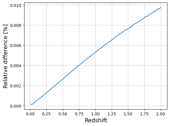
Sanity Checks - compare the CCL and NC implementations

Volume element

z_arr = np.linspace(0.01, 2, 100)
v_nc = [mf.dv_dzdomega(cosmo_nc, z) for z in z_arr]
v_ccl = dV_over_dOmega_dz(z_arr)
plt.plot(z_arr, np.abs(v_nc / v_ccl - 1) * 100)
plt.xlabel("Redshift", size=14)
plt.ylabel("Relative difference [%]", size=14)
plt.grid(which="major", lw=0.5)
plt.grid(which="minor", lw=0.2)

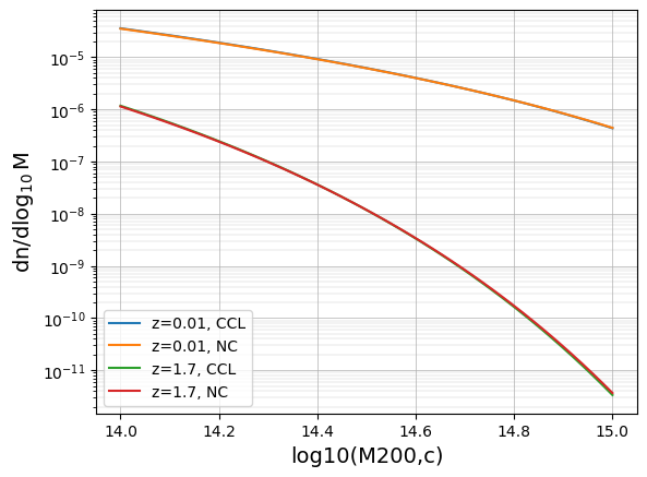
Mass function

The CCL and Numcosmo implementations give different results for the Tinker08 HMF, especially at high redshift (>1.5). Need to understand why, although it is not a regime we should find ourselves in with cluster studies at optical wavelength. Might be that the CCL and NC cosmologies defined above are not actually the same (neutrinos?).

logm_arr = np.linspace(14.0, 15)
z_arr = np.linspace(0.01, 1.7, 2)

t08_vec_ccl = np.vectorize(tinker08_ccl)
t08_vec_nc = np.vectorize(tinker08_nc)
for z in z_arr:
    res_ccl = t08_vec_ccl(logm_arr, z)
    res_nc = t08_vec_nc(logm_arr, z)
    plt.plot(logm_arr, res_ccl, label=f"z={z}, CCL")
    plt.plot(logm_arr, res_nc, label=f"z={z}, NC")
    plt.yscale("log")
    plt.xlabel("log10(M200,c)", size=14)
    plt.ylabel("dn/d$\log_{10}$M", size=14)
plt.legend()
plt.grid(which="major", lw=0.5)
plt.grid(which="minor", lw=0.2)

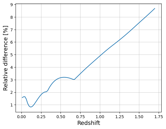
z_arr = np.linspace(0.01, 1.7, 100)
logm = 15.0
res_ccl = t08_vec_ccl(logm, z_arr)
res_nc = t08_vec_nc(logm, z_arr)
plt.plot(z_arr, np.abs(res_ccl / res_nc - 1) * 100)
plt.xlabel("Redshift", size=14)
plt.ylabel("Relative difference [%]", size=14)
plt.grid(which="major", lw=0.5)
plt.grid(which="minor", lw=0.2)

Acceptance-rejection method to sample (M,z) from the mass function

def bivariate_draw(
    pdf, N=1000, logm_min=14.0, logm_max=15.0, zmin=0.01, zmax=1, Ngrid_m=30, Ngrid_z=30
):
    """
    Uses the rejection method for generating random numbers derived from an arbitrary
    probability distribution.

    Parameters
    ----------
    pdf : func
      2d distribution function to sample
    N : int
      number of points to generate
    log_min,logm_max : float
      log10 mass range
    zmin,zmax : float
      redshift range

    Returns:
    --------
    ran_logm : list
        accepted logm values
    ran_z : list
        accepted redshift values
    acceptance : float
        acceptance ratio of the method
    """

    # maximum value of the pdf over the mass and redshift space.
    # the pdf is not monotonous in mass and redshift, so we need
    # to find the maximum numerically. Here we scan the space
    # with a regular grid and use the maximum value.
    # Accuracy of the results depends on Ngrid_m and Ngrid_z
    # This should probably be improved

    logM_arr = np.linspace(logm_min, logm_max, Ngrid_m)
    z_arr = np.logspace(np.log10(zmin), np.log10(zmax), Ngrid_z)
    p = []
    for logM in logM_arr:
        for z in z_arr:
            p.append(pdf(logM, z))
    pmax = np.max(p)
    pmin = np.min(p)
    # Counters
    naccept = 0
    ntrial = 0

    # Keeps drawing until N points are accepted
    ran_logm = []  # output list of random numbers
    ran_z = []  # output list of random numbers
    while naccept < N:
        # draw (logm,z) from uniform distribution
        # draw p from uniform distribution
        logm = np.random.uniform(logm_min, logm_max)  # x'
        z = np.random.uniform(zmin, zmax)  # x'
        p = np.random.uniform(0.0, pmax)  # y'

        if p < pdf(logm, z):
            # keep the point
            #            print(logm, z, p, pdf(logm, z))
            ran_logm.append(logm)
            ran_z.append(z)
            naccept = naccept + 1
        ntrial = ntrial + 1

    ran_logm = np.asarray(ran_logm)
    ran_z = np.asarray(ran_z)

    acceptance = float(N / ntrial)
    print(f"acceptance = {acceptance}")
    return ran_logm, ran_z, acceptance

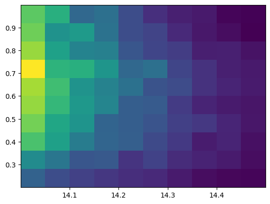
Draw \(10^4\) (M,z) pairs and check consistency with mass function

# Define the numbers of pairs to draw and the mass and redshift ranges
N = 10000
logm_min = 14.0
logm_max = 14.5
zmin = 0.2
zmax = 1.0

# Choose between the CCL and NC implementation (NC is faster)
# pdf = pdf_tinker08_ccl
pdf = pdf_tinker08_nc

# Normalisation factor for the pdf to be used later
norm = (
    1.0
    / scipy.integrate.dblquad(
        pdf, zmin, zmax, lambda x: logm_min, lambda x: logm_max, epsrel=1.0e-4
    )[0]
)

# Random draw
ran_logm, ran_z, acceptance = bivariate_draw(
    pdf, N=N, logm_min=logm_min, logm_max=logm_max, zmin=zmin, zmax=zmax
)

acceptance = 0.32901230506020923

plt.hist2d(ran_logm, ran_z, bins=10)
pass

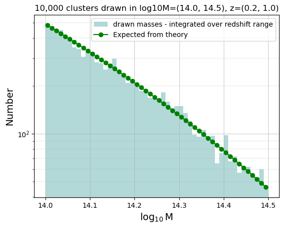
Check distribution in mass bins (integrate over the full redshift range)

hist_m = np.histogram(ran_logm, bins=50)

print(zmin, zmax)
predicted_T08_m_quad = [
    norm
    * N
    * scipy.integrate.dblquad(pdf, zmin, zmax, lambda x: lmmin, lambda x: lmmax, epsrel=1.0e-4)[0]
    for lmmin, lmmax in zip(hist_m[1], hist_m[1][1:])
]

0.2 1.0

bin_centers_m = 0.5 * (hist_m[1][:-1] + hist_m[1][1:])

plt.hist(
    ran_logm,
    bins=hist_m[1],
    color="teal",
    alpha=0.3,
    label="drawn masses - integrated over redshift range",
)
plt.plot(
    bin_centers_m, np.array(predicted_T08_m_quad), "-o", color="green", label="Expected from theory"
)
plt.yscale("log")
plt.xlabel("$\log_{10}$M", size=14)
plt.ylabel("Number", size=14)
plt.title(f"{N:,} clusters drawn in log10M={logm_min, logm_max}, z={zmin, zmax}")
plt.legend()
plt.grid(which="major", lw=0.5)
plt.grid(which="minor", lw=0.2)

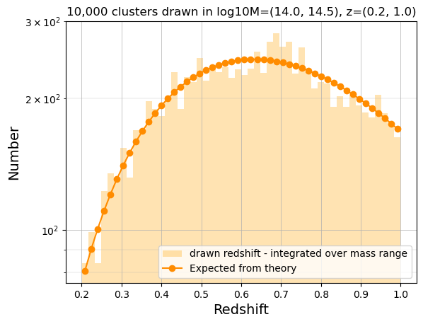
Check distribution in redshift bins (integrate over the full mass range)

hist_z = np.histogram(ran_z, bins=50)

print(logm_min, logm_max)
predicted_T08_z_quad = [
    norm
    * N
    * scipy.integrate.dblquad(
        pdf, zzmin, zzmax, lambda x: logm_min, lambda x: logm_max, epsrel=1.0e-4
    )[0]
    for zzmin, zzmax in zip(hist_z[1], hist_z[1][1:])
]

14.0 14.5

bin_centers_z = 0.5 * (hist_z[1][:-1] + hist_z[1][1:])

plt.hist(
    ran_z,
    bins=hist_z[1],
    color="orange",
    alpha=0.3,
    label="drawn redshift - integrated over mass range",
)
plt.plot(
    bin_centers_z,
    np.array(predicted_T08_z_quad),
    "-o",
    color="darkorange",
    label="Expected from theory",
)
plt.yscale("log")
plt.xlabel("Redshift", size=14)
plt.ylabel("Number", size=14)
plt.title(f"{N:,} clusters drawn in log10M={logm_min, logm_max}, z={zmin, zmax}")
plt.legend(loc=4)
plt.grid(which="major", lw=0.5)
plt.grid(which="minor", lw=0.2)

Generating a cluster catalog and associated source catalogs

• First, set the cluster masses and redshifts given the generated mock data. Only keep 30 clusters from N generated above to avoid memory issues.

• Then, instantiate a CCL concentration object to compute the concentration for each cluster from a mass-concentration realtion (Duffy et al. 2008). The actual concentration for each cluster is drawn from a lognormal distribution around the mean value

• Last, we randomly generate the cluster center coordinates over the full sky (from 0 to 360 deg for ra and from -90 to 90 deg to dec)

Cluster ensemble masses, redshifts and positions

# Randomly keep 30 (M,z) pairs from the 1000s generated abve.
Nstack = 30
indices = np.random.choice(len(ran_logm), Nstack)
cluster_m = 10 ** ran_logm[indices]
cluster_z = ran_z[indices]

# Concentration CCL object to compute the theoretical concentration
conc_obj = ccl.halos.ConcentrationDuffy08(mass_def=hmd_200c)
conc_list = []
for number in range(0, len(cluster_m)):
    a = 1.0 / (1.0 + (cluster_z[number]))
    # mean value of the concentration for that cluster
    lnc_mean = np.log(conc_obj(cosmo, M=(cluster_m[number]), a=a))
    # random draw of actual concentration from normal distribution around lnc_mean, with a 0.14 scatter
    lnc = np.random.normal(lnc_mean, 0.14)
    conc_list.append(np.exp(lnc))

conc_list = np.array(conc_list)

# randomly draw cluster positions over the full sky
ra = np.random.random(N) * 360  # from 0 to 360 deg
sindec = np.random.random(N) * 2 - 1
dec = np.arcsin(sindec) * 180 / np.pi  # from -90 to 90 deg

len(cluster_m)
Nstack

30

Background galaxy catalog generation

For each cluster of the ensemble, we use mock_data to generate a background galaxy catalog and store the results in a GalaxyCluster object. Note that: - The cluster density profiles follow the NFW parametrisation - The source redshifts follow the Chang et al. distribution and have associated pdfs - The shapes include shape noise and shape measurement errors - Background galaxy catalogs are independent, even if the clusters are close (i.e., no common galaxy between two catalogs). - For each cluster we then compute - the tangential and cross \(\Delta\Sigma\) for each background galaxy - the weights w_ls to be used to compute the corresponding radial profiles (see demo_compute_deltasigma_weights.ipynb notebook for details)

The cluster objects are then stored in gclist.

import warnings

warnings.simplefilter(
    "ignore"
)  # just to prevent warning print out when looping over the cluster ensemble below

%%time
gclist = []
# number of galaxies in each cluster field (alternatively, can use the galaxy density instead)
n_gals = 10000
# ngal_density = 10
cosmo_clmm = Cosmology(H0=71.0, Omega_dm0=0.265 - 0.0448, Omega_b0=0.0448, Omega_k0=0.0)
# cosmo_clmm.set_be_cosmo(cosmo)
gal_args = dict(
    cosmo=cosmo_clmm,
    zsrc="chang13",
    delta_so=200,
    massdef="critical",
    halo_profile_model="nfw",
    zsrc_max=3.0,
    field_size=10.0,
    shapenoise=0.04,
    photoz_sigma_unscaled=0.02,
    ngals=n_gals,
    mean_e_err=0.1,
)

for i in range(Nstack):
    # generate background galaxy catalog for cluster i
    cl = clmm.GalaxyCluster(
        f"mock_cluster_{i:04}",
        ra[i],
        dec[i],
        cluster_z[i],
        galcat=mock.generate_galaxy_catalog(
            cluster_m[i],
            cluster_z[i],
            conc_list[i],
            cluster_ra=ra[i],
            cluster_dec=dec[i],
            zsrc_min=cluster_z[i] + 0.1,
            **gal_args,
        ),
    )

    # compute DeltaSigma for each background galaxy
    cl.compute_tangential_and_cross_components(
        shape_component1="e1",
        shape_component2="e2",
        tan_component="DS_t",
        cross_component="DS_x",
        cosmo=cosmo_clmm,
        is_deltasigma=True,
        use_pdz=True,
    )

    # compute the weights to be used to bluid the DeltaSigma radial profiles
    cl.compute_galaxy_weights(
        use_pdz=True,
        use_shape_noise=True,
        shape_component1="e1",
        shape_component2="e2",
        use_shape_error=True,
        shape_component1_err="e_err",
        shape_component2_err="e_err",
        weight_name="w_ls",
        cosmo=cosmo_clmm,
        is_deltasigma=True,
        add=True,
    )

    # append the cluster in the list
    gclist.append(cl)

CPU times: user 1.68 s, sys: 280 ms, total: 1.96 s
Wall time: 1.96 s

cl.galcat.columns

<TableColumns names=('ra','dec','e1','e2','e_err','z','ztrue','pzpdf','id','sigma_c_eff','theta','DS_t','DS_x','w_ls')>

Creating ClusterEnsemble object and estimation of individual excess surface density profiles

From the galaxy cluster object list gclist, we instantiate a cluster ensemble object clusterensemble. This instantiation step uses - the individual galaxy input \(\Delta\Sigma_+\) and \(\Delta\Sigma_{\times}\) values (computed in the previous step, DS_{t,x}) - the corresponding individual input weights w_ls (computed in the previous step)

to compute

• the output tangential DS_t and cross signal DS_x binned profiles (where the binning is controlled by bins)

• the associated profile weights W_l (that will be used to compute the stacked profile)

%%time
ensemble_id = 1
bins = np.logspace(np.log10(0.3), np.log10(5), 10)
clusterensemble = ClusterEnsemble(
    ensemble_id,
    gclist,
    tan_component_in="DS_t",
    cross_component_in="DS_x",
    tan_component_out="DS_t",
    cross_component_out="DS_x",
    weights_in="w_ls",
    weights_out="W_l",
    bins=bins,
    bin_units="Mpc",
    cosmo=cosmo_clmm,
)

CPU times: user 280 ms, sys: 0 ns, total: 280 ms
Wall time: 280 ms

There is also the option to create an ClusterEnsemble object without the clusters list. Then, the user may compute the individual profile for each wanted cluster and compute the radial profile once all the indvidual profiles have been computed. This method may be reccomended if there a large number of clusters to avoid excess of memory allocation, since the user can generate each cluster separately, compute its individual profile and then delete the cluster object.

ensemble_id2 = 2
empty_cluster_ensemble = ClusterEnsemble(ensemble_id2)
for cluster in gclist:
    empty_cluster_ensemble.make_individual_radial_profile(
        galaxycluster=cluster,
        tan_component_in="DS_t",
        cross_component_in="DS_x",
        tan_component_out="DS_t",
        cross_component_out="DS_x",
        weights_in="w_ls",
        weights_out="W_l",
        bins=bins,
        bin_units="Mpc",
        cosmo=cosmo_clmm,
    )

A third option is where all clusters already have the profile computed, and we just add those to the ClusterEnsemble object:

# add profiles to gclist
for cluster in gclist:
    cluster.make_radial_profile(
        tan_component_in="DS_t",
        cross_component_in="DS_x",
        tan_component_out="DS_t",
        cross_component_out="DS_x",
        weights_in="w_ls",
        weights_out="W_l",
        bins=bins,
        bin_units="Mpc",
        cosmo=cosmo_clmm,
    )

ensemble_id3 = 3
empty_cluster_ensemble = ClusterEnsemble(ensemble_id3)
for cluster in gclist:
    empty_cluster_ensemble.add_individual_radial_profile(
        galaxycluster=cluster,
        profile_table=cluster.profile,
        tan_component="DS_t",
        cross_component="DS_x",
        weights="W_l",
    )

Stacked profile of the cluster ensemble

The stacked radial profile of the ensemble is then obtained as

clusterensemble.make_stacked_radial_profile(tan_component="DS_t", cross_component="DS_x")

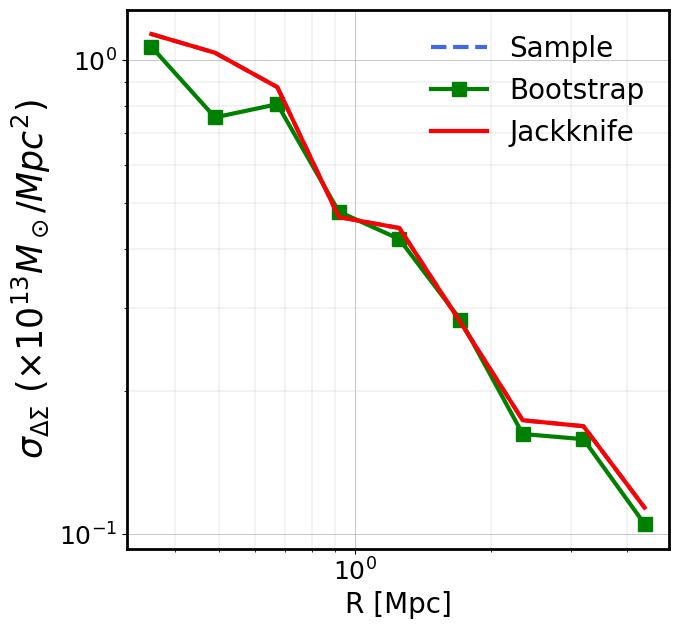
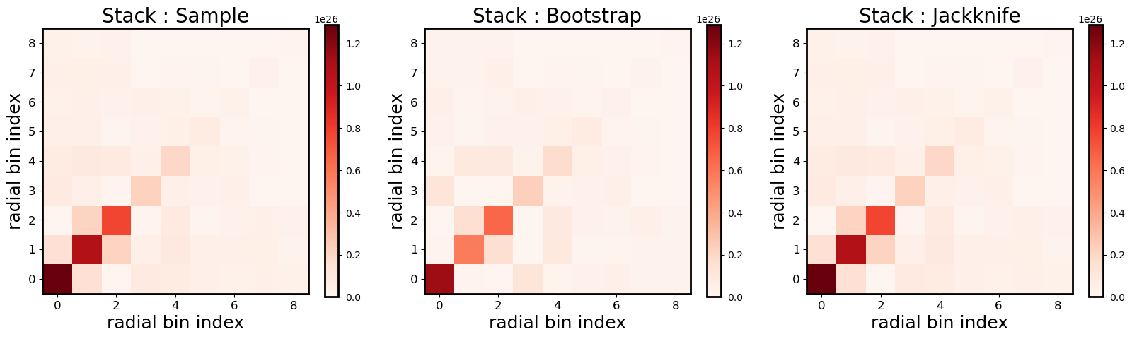
Covariance (Bootstrap, sample, Jackknife) of the stack between radial bins

Radial bins may be correlated and the ClusterEnsemble class provides three methods to compute the covariance matrix of the stacked signal, from the data: - The Sample covariance directly computes the covariance between radial bins of the N individual cluster profiles of the stack. - The Bootstrap approach is a resampling technique generating n_bootstrap ensembles of N randomly drawn clusters from the original ensemble, allowing for duplication. For each new ensemble, the stacked profile is computed and the covariance computed over the n_bootstrap stacks. - The Jackknife approach is another resampling technique, that divides the sky in a given number of regions \(N_{\rm region}\) and computes the covariance removing one region (i.e the clusters of the ensemble in that region) at a time. The stack is then computed using the remaining clusters and the covariance computed over the \(N_{\rm region}\) number of stacks. The division of the sky is done using the Healpix pixelisation scheme and is controlled by the n_side parameter, with \(N_{\rm region}=12 N_{\rm side}^2\).

NB: Approaches exist to compute the theoretical covariance of a stack but these are not (yet) available in CLMM

clusterensemble.compute_sample_covariance(tan_component="DS_t", cross_component="DS_x")
clusterensemble.compute_bootstrap_covariance(
    tan_component="DS_t", cross_component="DS_x", n_bootstrap=300
)
clusterensemble.compute_jackknife_covariance(
    n_side=16, tan_component="DS_t", cross_component="DS_x"
)

plt.figure(figsize=(7, 7))
plt.rcParams["axes.linewidth"] = 2
plt.plot(
    clusterensemble.data["radius"][0],
    clusterensemble.cov["tan_sc"].diagonal() ** 0.5 / 1e13,
    "--",
    c="royalblue",
    label="Sample",
    linewidth=3,
)
plt.plot(
    clusterensemble.data["radius"][0],
    clusterensemble.cov["tan_jk"].diagonal() ** 0.5 / 1e13,
    "-s",
    c="g",
    label="Bootstrap",
    linewidth=3,
    markersize=10,
)
plt.plot(
    clusterensemble.data["radius"][0],
    clusterensemble.cov["tan_sc"].diagonal() ** 0.5 / 1e13,
    c="r",
    label="Jackknife",
    linewidth=3,
)
plt.xlabel("R [Mpc]", fontsize=20)
plt.ylabel(r"$\sigma_{\Delta\Sigma}\ (\times 10^{13} M_\odot /Mpc^2)$", fontsize=25)
plt.tick_params(axis="both", which="major", labelsize=18)
plt.legend(frameon=False, fontsize=20)
plt.loglog()
plt.grid(which="major", lw=0.5)
plt.grid(which="minor", lw=0.2)

fig, axes = plt.subplots(1, 3, figsize=(20, 5))
plt.rcParams["axes.linewidth"] = 2
fig.subplots_adjust(wspace=0.15, hspace=0)

maximum = clusterensemble.cov["tan_sc"].max()
for ax, cov, label in zip(
    axes,
    [clusterensemble.cov["tan_sc"], clusterensemble.cov["tan_jk"], clusterensemble.cov["tan_sc"]],
    ["Stack : Sample", "Stack : Bootstrap", "Stack : Jackknife"],
):
    ax.set_title(label, fontsize=20)
    ax.set_xlabel("radial bin index", fontsize=18)
    ax.set_ylabel("radial bin index", fontsize=18)
    ax.tick_params(axis="both", which="major", labelsize=12)
    im = ax.imshow(cov, cmap="Reds", vmin=0, vmax=maximum, origin="lower")
    plt.colorbar(im, ax=ax)

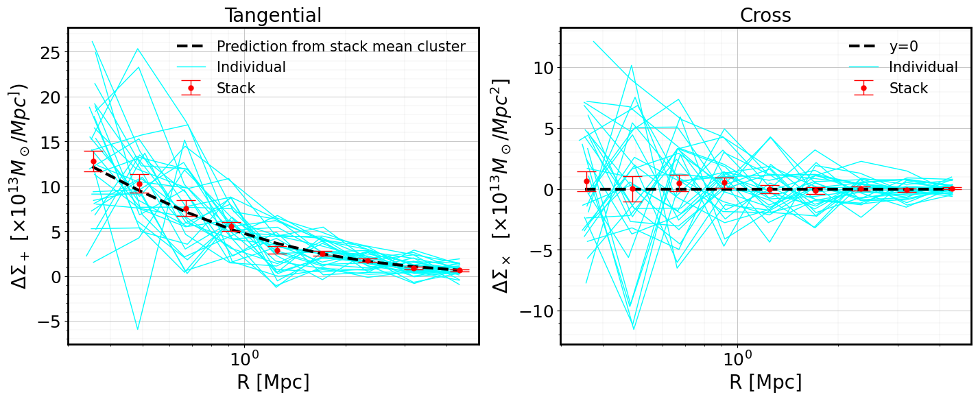
Visualizing the stacked profiles and corresponding model

In the figure below, we plot: - the individual \(\Delta\Sigma\) profiles of the clusters (light blue) - the stacked signal (red symbols) - the prediction computed using a NFW profile and the mean values of the mass, concentration and redshift in the stack (dashed black)

moo = clmm.Modeling(massdef="critical", delta_mdef=200, halo_profile_model="nfw")
moo.set_cosmo(cosmo_clmm)
# Average values of mass and concentration of the ensemble to be used below
# to overplot the model on the stacked profile
moo.set_concentration(conc_list.mean())
moo.set_mass(cluster_m.mean())

r_stack, gt_stack, gx_stack = (clusterensemble.stacked_data[c] for c in ("radius", "DS_t", "DS_x"))
plt.rcParams["axes.linewidth"] = 2
fig, axs = plt.subplots(1, 2, figsize=(17, 6))

err_gt = clusterensemble.cov["tan_sc"].diagonal() ** 0.5 / 1e13
err_gx = clusterensemble.cov["cross_sc"].diagonal() ** 0.5 / 1e13

axs[0].errorbar(
    r_stack,
    gt_stack / 1e13,
    err_gt,
    markersize=5,
    c="r",
    fmt="o",
    capsize=10,
    elinewidth=1,
    zorder=1000,
    alpha=1,
    label="Stack",
)
axs[1].errorbar(
    r_stack,
    gx_stack / 1e13,
    err_gx,
    markersize=5,
    c="r",
    fmt="o",
    capsize=10,
    elinewidth=1,
    zorder=1000,
    alpha=1,
    label="Stack",
)
# print(moo.eval_excess_surface_density(clusterensemble.data['radius'][0], cluster_z.mean())/1e13)
axs[0].plot(
    clusterensemble.data["radius"][0],
    moo.eval_excess_surface_density(clusterensemble.data["radius"][0], cluster_z.mean()) / 1e13,
    "--k",
    linewidth=3,
    label="Prediction from stack mean cluster",
    zorder=100,
)
axs[1].plot(
    clusterensemble.data["radius"][0],
    0 * moo.eval_excess_surface_density(clusterensemble.data["radius"][0], cluster_z.mean()) / 1e13,
    "--k",
    linewidth=3,
    label="y=0",
    zorder=100,
)

axs[0].set_xscale("log")
axs[1].set_xscale("log")


for i in range(Nstack):
    axs[0].plot(
        clusterensemble.data["radius"][i],
        clusterensemble.data["DS_t"][i] / 1e13,
        color="cyan",
        label="Individual",
        alpha=1,
        linewidth=1,
    )
    axs[1].plot(
        clusterensemble.data["radius"][i],
        clusterensemble.data["DS_x"][i] / 1e13,
        color="cyan",
        label="Individual",
        alpha=1,
        linewidth=1,
    )
    if i == 0:
        axs[0].legend(frameon=False, fontsize=15)
        axs[1].legend(frameon=False, fontsize=15)
# axs[0].plot(np.average(clusterensemble.data['radius'], axis = 0), np.average(clusterensemble.data['gt'], weights = None, axis = 0)/1e13)
axs[0].set_xlabel("R [Mpc]", fontsize=20)
axs[1].set_xlabel("R [Mpc]", fontsize=20)
axs[0].tick_params(axis="both", which="major", labelsize=18)
axs[1].tick_params(axis="both", which="major", labelsize=18)
axs[0].set_ylabel(r"$\Delta\Sigma_+$ $[\times 10^{13} M_\odot /Mpc^])$", fontsize=20)
axs[1].set_ylabel(r"$\Delta\Sigma_\times$  $[\times 10^{13} M_\odot /Mpc^2]$", fontsize=20)
axs[0].set_title(r"Tangential", fontsize=20)
axs[1].set_title(r"Cross", fontsize=20)

for ax in axs:
    ax.minorticks_on()
    ax.grid(lw=0.5)
    ax.grid(which="minor", lw=0.1)
plt.show()

Saving/Loading ClusterEnsemble

The ClusterEnsemble object also have an option for saving/loading:

clusterensemble.save("ce.pkl")

clusterensemble2 = ClusterEnsemble.load("ce.pkl")